Diffuse lighting

In the previous chapter we finally learned depth buffering, and that covered the basics of the Vulkan API and 3D rendering.

In this chapter we get started with lighting.

We will need to simulate lighting in our 3D scene, and to do that we will learn about the physics behind lighting. We will learn about a theoretical rendering equation and we will specialize it for direcr illumination, point lights and diffuse lighting. This will be a good foundation for real time rendering.

Then we will need to fill our swapchain images with RGB pixel data based on the simulated physical quantities, and to do that we will learn about physically based cameras, exposure correction, tonemapping and gamma correction.

After studying the theory, we will extend our depth buffered 3D application from the previous chapter to perform lighting calculations using the specialized rendering equation, and write RGB pixel data to the swapchain image derived from its results.

This tutorial is math and physics heavy and assumes you already have some intuition for calculus. The recommendations from the previous tutorials for consuming math still apply: you can understand math in many ways, depending on your way of thinking and background:

Read and understand the math first, then the code
Understand the code first, and then interpret the math

Read whichever way is better for you. Be prepared that multiple rereads may be necessary.

This tutorial is in open beta. There may be bugs in the code and misinformation and inaccuracies in the text. If you find any, feel free to open a ticket on the repo of the code samples.

Radiometry and the Rendering equation

Physically based rendering is about calculating how light ends up in the camera using equations derived from physics. Light is electromagnetic radiation described by a branch of physics called electrodynamics. Practicioners of computer graphics tend not to use Maxwell's equations directly, but instead introduce layers of abstractions and run simulations using much simpler equations than Maxwell's equations.

This section briefly summarizes the physics behind rendering. The human eye and cameras detect energy from light. We will introduce a physical quantity related to energy that we can use to determine the brightness of pixels, and an equation we can use to calculate the said physical quantity for every pixel based on how light travels from light sources through the scene to the camera.

This section is based on the computer graphics course of Two Minute Papers youtube channel.

Radiance

The brightness of the pixel is going to be calculated based on a physical quantity related to energy, but what is this physical quantity? This is explored in the aforementioned computer graphics course's Radiometry video.

There is a physical quantity called the radiant power measured in Watts $(W)$ . This is not good enough because of ambiguity: is there a small amount of power coming from a large surface or a large amount coming from a small surface? The amount of radiant power that we measure would be the same, but the distribution of the radiant power would be way different.

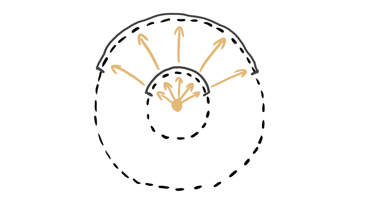
**Figure 1:** Illustration of the same radiant power distributed across different surfaces. The outer surface is much larger than the inner one, and it can radiate the same amount of power, but the energy distribution across the surface may be very different.

Let's try to get rid of the ambiguity! Let's get the radiant power per unit area! This is called irradiance and it's measured in Watts per square meter $(\frac{W}{m^{2}})$ . This is still not good enough because of ambiguity: is there a large amount of power coming from a large solid angle or a small amount coming from a small solid angle?

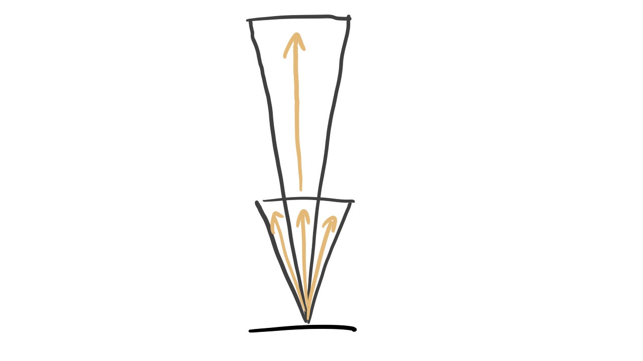
**Figure 2:** Illustration of surface with some irradiance radiating energy in different solid angles. The inner cone is smaller, and the energy radiated in it is smaller than the outer one, even though it's the same surface with the same irradiance.

Let's follow the same idea and try to get the radiant power per area per solid angle! This is called radiance and it's measured in Watts per steradian per square meter $(\frac{W}{sr \cdot m^{2}})$ . This finally removes all of the ambiguities.

Rendering equation

We have our physical quantity, radiance. Now we need equations that help us simulate how much radiance ends up in a pixel of our swapchain image.

We use a probabilistic model. We assume that incoming light coming from one direction can get reflected in many directions with certain probabilities, or may get absorbed by the surface. If we are curious about a certain direction, such as the direction of the camera, the probability tells us how much of the incoming radiance gets reflected towards the camera.

The equation starts to get introduced in the previously mentioned video, but only this one starts to get into details we need. The equation that we need to calculate the emitted light in terms of the incoming light is introduced below.

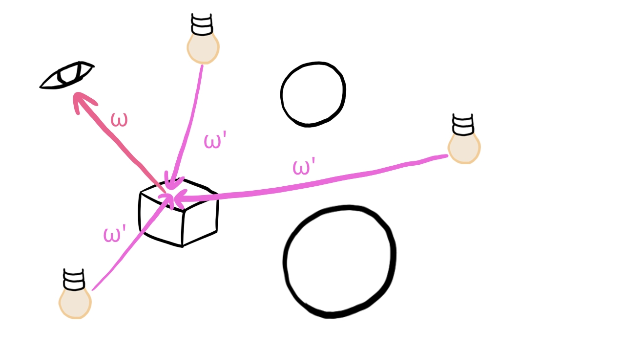
Let our surface element that covers a pixel be at point $x$ and let the direction vector pointing from the surface to the camera be $ω$ ! We want to figure our what $L_{o}$ radiance leaves the surface from point $x$ to direction $ω$ . The value of this $L_{o}$ radiance is given by the following equation called the Rendering equation.

L_{o} (x, ω, λ) = L_{e} (x, ω, λ) + \int_{Ω}^{} L_{i} (x, ω', λ) \cdot f (ω, x, ω', λ) \cdot \cos (θ_{n, ω'}) d ω'

The radiance $L_{o}$ equals to the sum of the emitted radiance $L_{e}$ emitted by the surface and the reflected radiance. The reflected radiance for a given $ω'$ equals to the sum of incoming radiance $L_{i}$ from this $ω'$ direction, multiplied by a probability density function $f$ that gives the probability of the surface at point $x$ reflecting light from direction $ω'$ to direction $ω$ , weighted by the surface element's projected area. This probability function is called Bidirectional reflectance distribution function. You see that there is a multiplication inside the integral with the cosine of the angle $θ_{n, ω'}$ , which is the angle between the $ω'$ direction and the surface's $n$ normal at point $x$ . This cosine is the scaling factor between the surface element's projected area at point $x$ and the actual area. We need to sum this up to the whole $Ω$ hemisphere. In our model the $Ω$ hemisphere contains infinite $ω'$ directions continuously, so summing up the reflected radiance for all of these directions is done using an integral.

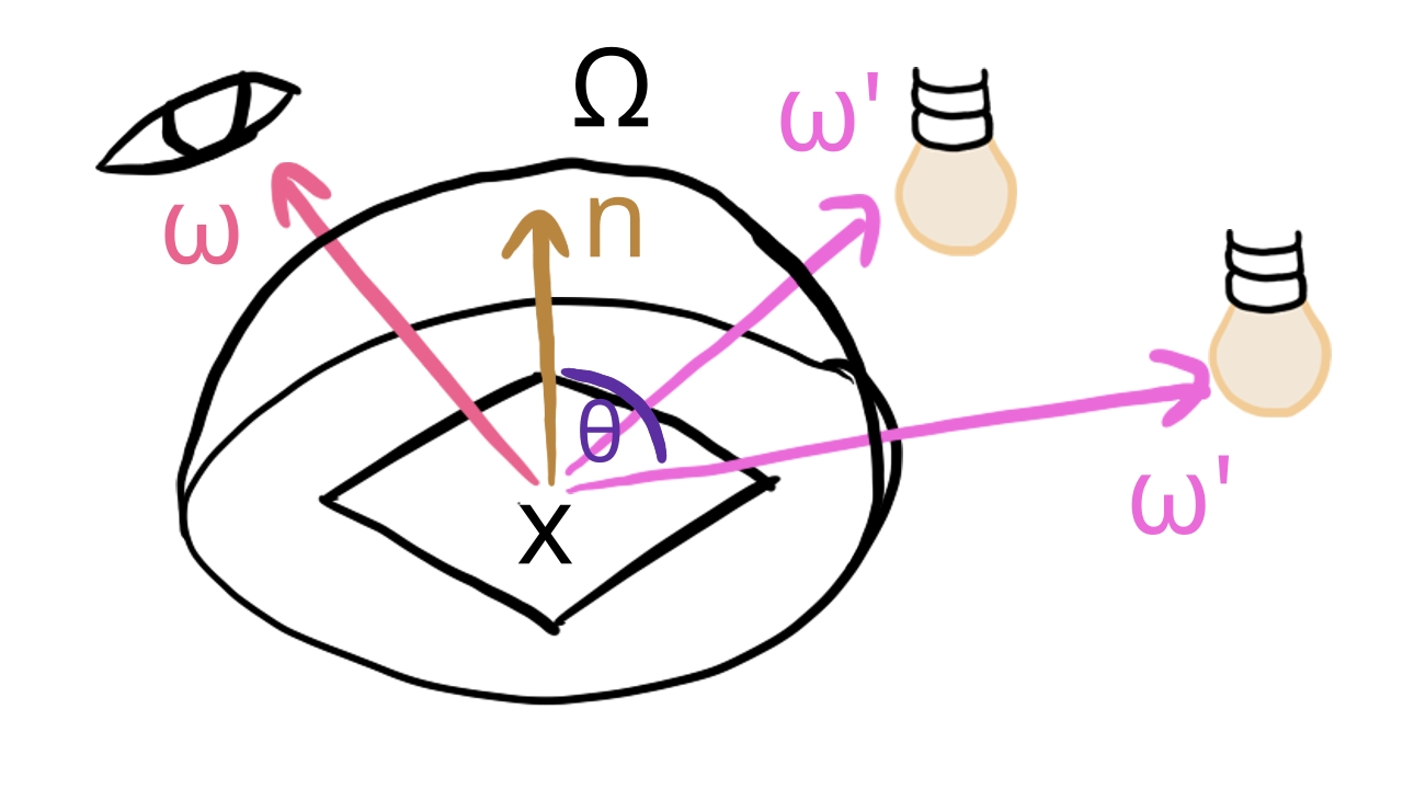
**Figure 3:** Illustration of some parameters of the rendering equation. The surface element is at position $x$ , $ω$ is the unit vector from position $x$ to the camera, $n$ is the normal vector of the surface, $Ω$ is the whole hemisphere of directions where radiance can come from, the $ω'$ vectors are all of the vectors within the $Ω$ hemisphere, and θn,ω′ is the angle between a given $ω'$ vector and the $n$ normal vector.

This equation is actually an infinite recursive equation, as the incoming radiance for every direction $φ$ leaves a surface element at point $x'$ also calculated by the Rendering equation.

L_{i} (x, φ, λ) = L_{o} (x', φ, λ) = L_{e} (x', φ, λ) + \int_{Φ}^{} L_{i_{2}} (x', φ', λ) \cdot f (φ, x', φ', λ) \cdot \cos (θ_{n, φ'}) d φ'

**Figure 4:** Illustration of the recursive nature of the rendering equation. Notice how the radiance coming from the $ω'$ directions all depend on incoming radiances coming from $φ'$ directions, all of them being given by a rendering equation.

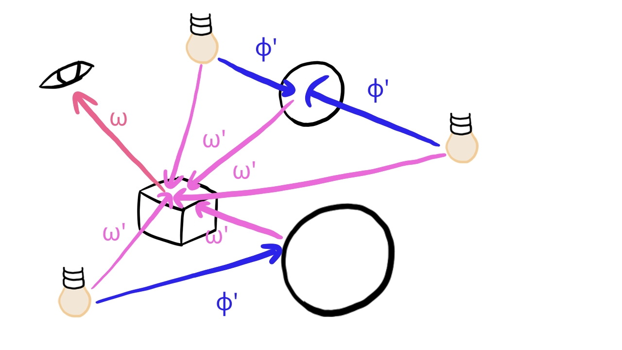
Such integrals cannot be evaluated on our computers. We need to specialize this problem. In this tutorial are going to simplify this equation. We will solve a simplified version that is not infinitely recursive, not an integral and the probability density function is very simple.

Direct illumination

First we cut off our recursion. Generally light bounces around and sometimes light reflected from other scene elements illuminate a scene element visible in a certain pixel. The recursion accounts for that as well. It aggregates incoming radiance from many sources. Solving that problem is called global illumination. In this article we will not go into that. Instead the brightness of our pixels is only affected by the radiance coming from the light sources directly. Since we remove indirect lighting, the formula for the incoming radiance $L_{i}$ is simplified like this:

L_{i} (x, φ, λ) = L_{o} (x', φ, λ) = L_{e} (x', φ, λ)

This modified formula will only take emissive light from scene elements into account inside the integral. No light that bounces around will be taken into account.

Calculating this exactly would still be pretty computationally intensive, because we need to find the closest hit $x'$ along our direction $φ$ . We simplify this by cheating a lot.

We group our scene elements into two groups: objects and lights. Lights will not be rendered directly, but they will emit radiance. Objects will be rendered directly, and their surface will reflect radiance coming only from lights.

Basically objects will not reflect other objects' emitted radiance, only lights' emitted radiance. This gets rid of many interdependencies of the reflected radiances of scene elements and decreases the algorithmic complexity of lighting.

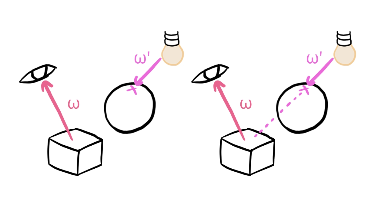
**Figure 5:** Illustration of direct illumination cutting off the recursion. Now that only illumination coming from lights are calculated, we do not need to calculate from many directions from many other surface elements recursively.

**Figure 6:** Illustration of removal of shadow casting removing interdependencies. If we do not need to check whether there is a scene object between the light source and the surface element along a given direction, we can calculate incoming radiance purely based on the surface element's data and the light data.

After this step we still have a bit of problem. Objects generally cast shadows, and to take that into account, we would have to find out when collecting radiance from a light if there is a triangle obstructing the light path. To get rid of this interdependency, objects will also not cast shadows. This will greatly decrease algorithmic complexity, because collecting the reflected radiance from light sources turns into a simple iteration over every light. In every iteration we collect a given light's contribution from the given direction. No need to check for occlusion by objects.

So far our incoming light equation looks like this:

L_{i} (x, φ, λ) = \sum_{\forall light}^{} L_{e} (x_{light}, φ, λ)

If an object covers a pixel, the color of the pixel will be determined by the model's emissive lighting and the incoming radiance of the light sources.

With these steps we have greatly decreased the complexity of our rendering equation, but there is still an integral in it, and without further assumptions a computer program still cannot be written to calculate it.

Point lights

In order to get rid of that integral we need some assumptions about our light sources.

If our light has a volume, we need to integrate for its whole surface. This is where point lights come in. Point lights emit light from a specific point, so no need to integrate over a surface.

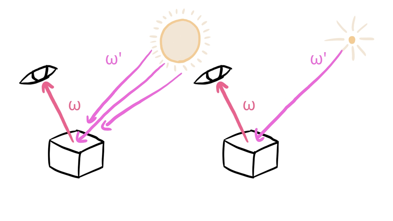
**Figure 7:** Comparison of area lights and point lights. Area lights emit light in the direction of a surface from many positions. Point lights on the other hand emit light in the direction of a surface only from one direction. This removes the need for integrating radiance for many directions.

Our integral and the choice of our units of measurement were prepared for light sources that have an area, but point lights do not have that. We need to figure out some hack to collect radiance contribution from our point light.

According to the PBR book it is incorrect to use radiance to describe the amount of light arriving at a point from a point light, and we should use the radiant intensity instead: the amount of radiant power exiting the light source per solid angle. We assume that based on this physical quantity the point light distributes radiance evenly in all directions.

I = \frac{Φ (λ)}{4 \cdot π}

The problem is that this is a different physical quantity with a different dimension. It contains the information needed to figure out how much energy the light source emits, but technically it is not directly usable.

How can we get from having $I$ to having something we can plug into our integral? There are multiple lines of thought that can build up the intuition for the formula used in the industry.

One is looking at other energy related physical quantities. For instance let's look at the irradiance $E$ :

E = \frac{Φ (λ)}{4 \cdot π \cdot r^{2}} = \frac{I (λ)}{r^{2}}

This is power per area. If the power of a point light gets evenly distributed across the surface of a sphere, this quantity would decrease with the inverse square of the radius. It is also a function of the radiant intensity. Its dimensions are also much friendlier than the dimension of radiant intensity.

This tells us that the amount of power coming from the point light to a surface element at distance $r$ decreases with the inverse square of $r$ . Our intuition should say that our "radiance" at distance $r$ should behave the same way.

There is a second line of thought trying to build up the same intuition. $I$ is the amount of radiant power per unit solid angle. Let's have a surface element with an area $A$ that is lit by our point light! How does the solid angle change if we increase the distance? According to Wikipedia, the solid angle is related to the area it cuts out from the sphere.

Ω = \frac{A}{r^{2}}

In our case $Ω$ is the solid angle, $A$ is the area of our surface and $r$ is the distance from our point light. Let's measure $A$ in square meters and $r$ in meters! If we choose our surface to have an area $A = 1 m^{2}$ , then the radiant power reaching the surface will be:

Φ (λ) = A \cdot \frac{I (λ)}{r^{2}} = 1 \cdot \frac{I (λ)}{r^{2}} = \frac{I (λ)}{r^{2}}

The formula looks very similar to the previous one but pay attention that the dimensions are not the same! What this is good enough is building up the intuition: the further we are, the radiant power reaching the surface will be proportional to the inverse square of the distance.

These ideas lead to the formula commonly used. If we divide $I$ by $r^{2}$ , we will get a physical quantity that has the same dimension as the radiance and will represent the amount of light decreasing with the inverse square of the distance.

L (λ) = \frac{I (λ)}{r^{2}}

We want to return this when the direction in the integral is the direction from the surface to the point light.

Let's construct a model for a single point light! We choose $L_{i} (x, ω', λ)$ to be a $\frac{I (λ)}{r^{2}} \cdot δ (ω' - ω_{l})$ "function", where $ω_{l}$ is the direction from the surface element to the point light, $r$ is the distance of point $x$ from the position of the point light and $δ (φ)$ is the Dirac delta. If we plug this $L$ into our integral, a single point light our integral simplifies the following way:

\int_{Ω}^{} L_{i} (x, ω', λ) \cdot f (ω, x, ω', λ) \cdot \cos (θ_{n, ω'}) d ω' = \int_{Ω}^{} \frac{I (λ)}{r^{2}} \cdot δ (ω' - ω_{l}) \cdot f (ω, x, ω', λ) \cdot \cos (θ_{n, ω'}) d ω' = \frac{I (λ)}{r^{2}} \cdot f (ω, x, ω_{l}, λ) \cdot \cos (θ_{n, ω_{l}})

The integral disappeared. Radiance from multiple lights is a simple sum.

\int_{Ω}^{} L_{i} (x, ω', λ) \cdot f (ω, x, ω', λ) \cdot \cos (θ_{n, ω'}) d ω' = \sum_{\forall light}^{} \frac{I_{l} (λ)}{{r_{l}}^{2}} \cdot f (ω, x, ω_{l}, λ) \cdot \cos (θ_{n,ω_{l}})

We have gotten far. No infinite recursion and no integral, but we still have an unknown function f, which is a function that determines what the probability of reflecting the radiance towards a given point is. We can choose this function for ourselves, so let's choose a popular one!

Diffuse BRDF

The $f$ BRDF function tells us what is the probability of a surface element at point $x$ reflecting light from light direction $ω'$ to the view direction $ω$ .

A very simple and widely used BRDF is the Lambertian model, which is suitable for perfectly matte surfaces. The Lambertien BRDF is the constant BRDF: it reflects light in every direction with equal probability. This probability may be small or large, depending on the probability of reflecting or absorbing light, but it is independent of the viewing angle.

How should we choose this constant $f$ function? We want it to be physically based, because we can handle that better in later tutorials. According to Wikipedia it should be larger than zero, and the integral of the function for the whole hemisphere should be less than one. In Epic's Real Shading in Unreal Engine 4 the diffuse BRDF is the following: let $ρ (λ)$ be the diffuse albedo of the material, $ρ (λ) \in [0, 1]$ . The diffuse BRDF will be:

f (ω, x, ω', λ) = \frac{ρ (λ)}{π}

We can plug this BRDF into our rendering equation and finally have something we can write in a shader.

Resulting simplified rendering equation

So far we have made the following assumptions:

We only calculate local illumination.
Objects do not cast shadow.
Out light sources will be point lights.
The BRDF of our objects will be Lambertian diffuse BRDF.

With these assumptions our simplified rendering equation looks like this:

L_{o} (x, ω, λ) = L_{e} (x, ω, λ) + \sum_{\forall light}^{} \frac{I_{l} (λ)}{{r_{l}}^{2}} \cdot \frac{ρ (λ)}{π} \cdot \cos (θ_{n,ω_{l}})

No infinite recursion, no integrals and we can calculate the color of every object using only its data and the list of lights affecting it. We are going to evaluate this formula for three wavelengths: the wavelength of the red color, the green color and the blue color. This way everything that is the function of $λ$ will become a number triplet.

Now that we have radiance, which can be anywhere from zero to infinity, we need to map it into the $[0, 1]$ range, because that's the range of values that can be stored in our swaphcain image. There are two things that need to be done to achieve this: first we do exposure compensation, and then do tone mapping.

Exposure correction

The human eye and cameras are all capable of forming images in both poorly lit and very well lit environments. Your pupil can get wider to let more light in when you are in a dark area, and narrower when you are in a well lit area. Cameras can collect more or less light as needed by adjusting the lens aperture or the shutter speed.

With this feature both the human eye and a camera can form a useful image in both dark caves and bight landscapes by controlling the amount of light entering the detector, visualizing dark areas lighter and light areas darker so they fall in the detectable range.

This process is called exposure correction. Exposure correction allows us to brighten or darken the image depending on the lighting conditions, instead of having to tweak the lights in the scene. It removes a lot of manual work. To perform exposure correction we need some kind of mathematical model that gives us formulae that we can write down as code. In this section we go over the A Physically Based Camera section of Moving Frostbite to PBR document. We introduce the concept of exposure for controlling the brightness of the resulting image, find the relationship between exposure and the maximum radiance of the image and calculate an exposure compensated radiance value that we can later map into the $[0, 1]$ interval in the next section.

Exposure is the amount of light per unit area reaching the sensor. A camera has the following parameters to control the exposure:

Relative aperture (f-number, N) controls how wide the aperture is opened.
Shutter time (t) controls how long the aperture is opened.
Sensor sensitivity (S) controls how photons are counted on the digital camera.

From these parameters the Exposure value can be calculated.

EV = \log_{2} (\frac{N^{2}}{t}) + \log_{2} (\frac{100}{S})

If $S = 100$ , we get ${EV}_{100}$ , which can be calculated using the following formula:

{EV}_{100} = \log_{2} (\frac{N^{2}}{t})

Now that we have these quantities, we need to figure out the formula that directly tells us the relationship between radiance and this exposure value. This is where another quantity called luminous exposure comes into play. The following formula can be found on Wikipedia:

H = \frac{q \cdot t}{N^{2}} \cdot L

Where $H$ is the luminous exposure, $L$ is the luminance of the scene and $q$ is the lens and vignetting attenuation.

This luminance is an energy related physical quantity, but it is not a radiometric quantity but a photometric quantity. Radiometry is a field of physics that deals with measuring electromagnetic radiation in general. Photometry on the other hand deals with measuring light in terms of its perceived brightness to the human eye. Many of their physical quantities are analogous to each other, but the units of measurement will be different. The Moving Frostbite to PBR document contains a table of radiometric and analogous photometric quantities in Table 5 of the Lighting section.

The photometric analogy of radiant power is luminous power. Because of ambiguities radiant power did not meet our requirements and we discovered radiance. The same problem occurs with luminous power, and we need to find a related quantity, which is luminance. Just as raidance is radiant power per area per solid angle, luminance is luminous power per area per solid angle. It is the photometric analogy of radiance and we will find a mathematical connection between them.

Now that we can grasp what luminance is, let's keep going with the formulae until we find the connection we need! There is a luminous exposure level $H_{sat}$ , which is the maximum possible luminous exposure that does not lead to a clipped or bloomed camera output. The following formula can be found on Wikipedia:

H_{sat} = \frac{78 \cdot lx \cdot s}{S}

We can substitute the formula for $H$ .

H_{sat} = \frac{q \cdot t}{N^{2}} \cdot L_{\max} = \frac{78 \cdot lx \cdot s}{S}

Now we can reorganize to get the max luminance.

L_{\max} = \frac{78 \cdot lx \cdot s}{S \cdot q} \cdot \frac{N^{2}}{t} = \frac{78 \cdot lx \cdot s}{S \cdot q} \cdot 2^{\log_{2} (\frac{N^{2}}{t})} = \frac{78 \cdot lx \cdot s}{S \cdot q} \cdot 2^{{EV}_{100}}

The Frostbite doc says that $S = 100$ and $q = 0.65$ is a good choice, so we have a direct relationship between ${EV}_{100}$ and the maximum luminance. Luminance can be converted to radiance by dividing with the maximum spectral luminous efficacy, which is $683 \frac{lm}{W}$ and now we have a relationship between radiance and the exposure value.

Related: Rendering equation with photometric quantities

If you feel pain while converting between radiometric and photometric quantities, you can just use photometric quantities. Instead of collecting radiance from the light sources, you can collect luminance. The rendering equation will work the same way, and the previous logical steps that we used to simplify the general rendering equation can be adapted, gaining a same looking equation, just with photometric quantities.

I chose radiometric quantities for the following reasons:

This is what the Two Minute Papers channel uses.
I assumed energy and power are more familiar from physics lessons.

You may find that artists are more familiar with luminance, so in a production application you may want to use luminance.

An exposure value can be calculated from the average luminance of the image as well. This can be useful for eye adaptation, which we will do in a later chapter. I recommend reading the A Physically Based Camera section of the Frostbite document to learn more.

Tone mapping

After exposure correction we have a number which tells us how bright the pixel should be, but the swapchain image with our setup can only contain color components in the $[0, 1]$ range. Tone mapping is the processing stage when we take the result of our rendering calculations, which fall in the range of $[0, \infty]$ , and map it to the range of $[0, 1]$ .

We could just clamp the result of the exposure correction step, because the value 1 would match the maximum luminance our camera can detect, but if we plug it into some curve the resulting image may be more pleasing to the eye. You can find some useful curves on Wikipedia.

In this tutorial we use the ACES curve from Krzysztof Narkowicz's blog post.

\begin{matrix} a = 2.51 \\ b = 0.03 \\ c = 2.43 \\ d = 0.59 \\ e = 0.14 \\ f (x) = \max (0.0, \min (1.0, \frac{x \cdot (a \cdot x + b)}{x \cdot (c \cdot x + d) + e})) \end{matrix}

Now the color value for each color component falls into the range of $[0, 1]$ , but we are still not done, because the swapchain's color space determines the interpretation of the pixel, so we must make sure that the value we write will be interpreted as the right color.

Linear to sRGB conversion

Now that we have tonemapped RGB values that fall within the range of $[0, 1]$ , we need to make sure that we write values that will be interpreted correctly. If the Swapchain image format is R8G8B8A8, then every color channel will be an integer value within the range of $[0, 255]$ , but the light intensity emitted by the monitor may not correspond to these values linearly. This will be determined by the swapchain's color space, which is set to VK_COLOR_SPACE_SRGB_NONLINEAR_KHR.

The rendering equation gave linear radiance values, and even after tone mapping there is a problem with them: many shades of grey cluster close to zero, and the mid-grey is very close to zero. In sRGB color space the mid-grey is placed in the middle of the interval, so the dark shades of grey are more spread out. This is a much better utilization of the $[0, 255]$ interval, because more precision is used for the shades of grey between black and the middle-grey. More details on the sRGB color space can be found on Wikipedia.

In order to convert from linear radiance values to sRGB is to plug it into the so called sRGB curve. The Frostbite document mentions at the Color Space section that there is an approximation to this curve, and warns against using it. The correct curve is the following:

sRGB (x) = {\begin{matrix} x \cdot 12.92 & x <= 0.0031308 \\ {| x |}^{\frac{1.0}{2.4}} \cdot 1.055 - 0.055 & x > 0.0031308 \end{matrix}

In this tutorial we will follow the recommendation and use the correct curve. Without transforming our tone mapped linear radiance value, the numbers we write to the swapchain image will be misinterpreted, and the whole image will be darker than it should be, so applying this function is necessary.

Now that we have covered all the theory we need, we can start figuring out our scene representation and get to coding.

Scene representation

In order to form images using the previously described method, we need to extend our scene representation to make sure it contains all the information our new formulae require. These will be surface normals, material data and light data.

The rendering equation requires surface normals to determine the projected surface area, so we need to add normals to our models' vertex data. For the normal vectors in-between vertices we will interpolate the normals assigned to the triangle vertices. Notice that this is a bit of cheating, because a triangle is a flat surface, and the normal vectors should be the same across the whole triangle, but allowing different normal vectors for every vertex and smoothly interpolating them for lighting calculations can be exploited to give the illusion of smooth surfaces.

**Figure 8:** Illustration of smooth normals. On the left you can see a single normal applied to every triangle. The problem is the sudden change between the normals along face boundary. When you apply the rendering equation, this will result in sudden changes of surface lightness along the face boundaries. On the right you can see that assigning different normals to different vertices, and interpolating normals between vertices results in smooth transition within triangles. When the rendering equation is applied to this arrangement, the surface lightness will change smoothly as well. If sharp changes and flat surfaces are desired, special data arrangement can solve that with smooth normals as well, as you can see with the cube data, but it allows arrangements with smooth transitions as well.

The rendering equation also depends on certain pieces of material data, so we need to add these to every scene object. Some of these are the parameters of the BRDF. In the case of the simple diffuse BRDF this is the probability of reflecting red, green and blue light, which will be three constants. We call these the albedo. Beyond these the material can emit light, and the parameters of this will be the emitted radiance for the red, green and blue components. We call this emissive light.

We will store the material data for every scene object separately. I chose this approach for this tutorial because it's simple and you have freedom in your game logic to continuously change a scene object's color if you want. For instance a scene objest's color can change from red to green, or from golden to silver continuously. The downside is the data duplication for scene objects that share the same material data, and the unnecessary data transfer for scene objects whose materials don't change. I chose this simple approach for learning, but you may want to implement something different in a real world application.

Finally we use the rendering equation to collect the radiance from direct illumination coming from a list of point lights, so we need to add these to the scene. They will be represented by their position in the scene, and the radiant intensity for the emitted red, green and blue light.

Now that we laid out what kind of data we need, we also need to talk about how this data will be processed. We will upload normals as vertex data, and it will be available in the vertex shader as an attribute. We will apply the necessary transformation and pass it to the fragment shader, just as we did with texture coordinates. Then the fragment shader will contain the implementation of the specialized rendering equation. It will have access to the normals passed from the vertex shader as an in variable, and it will need access to the material and light data to gather the radiance emitted and reflected by the surface element. After the radiance arriving at the camera at the given pixel is determined, we will apply exposure correction, tone mapping and sRGB conversion at the end of the fragment shader and write the results into the swapchain image.

Now that we have defined our tasks, it's time to start implementing them.

Adding normals to models

Data preparation

We need to add normals to our triangle and quad. These models are thin, and if you rotate the scene object, you will see its thin model from behind. We need to decide that one of its side is the front face, ant the other is the back face. The normal will point in the direction of the front face, and when the back face is seen, we just flip the normals. In this tutorial the front face will look at the positive Z direction in object space.

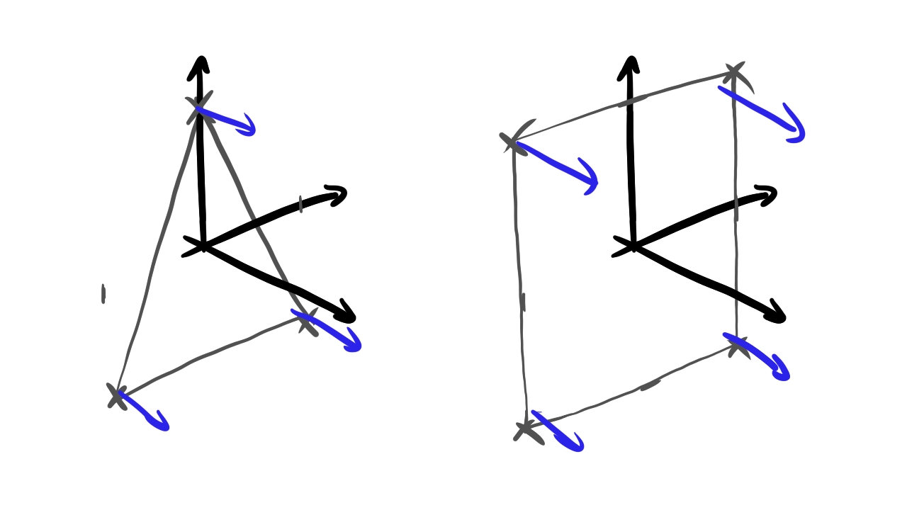
**Figure 9:** Illustration of the triangle and quad normals. The normal for every vertex points towards the positive z direction. When shaded this will look like a flat surface.

The new content of the array will be the following:


    vec![
        // Triangle
        //   Vertex 0
        -1.0, -1.0, 0.0,
        //   Normal 0
        0.0, 0.0, 1.0,
        //   TexCoord 0
        0.0, 0.0,
        //   Vertex 1
        1.0, -1.0, 0.0,
        //   Normal 1
        0.0, 0.0, 1.0,
        //   TexCoord 1
        1.0, 0.0,
        //   Vertex 2
        0.0,  1.0, 0.0,
        //   Normal 2
        0.0, 0.0, 1.0,
        //   TexCoord 2
        0.5, 1.0,
        // Quad
        //   Vertex 0
        -1.0, -1.0, 0.0,
        //   Normal 0
        0.0, 0.0, 1.0,
        //   TexCoord 0
        0.0, 0.0,
        //   Vertex 1
        1.0, -1.0, 0.0,
        //   Normal 1
        0.0, 0.0, 1.0,
        //   TexCoord 1
        1.0, 0.0,
        //   Vertex 2
        1.0, 1.0, 0.0,
        //   Normal 2
        0.0, 0.0, 1.0,
        //   TexCoord 2
        1.0, 1.0,
        //   Vertex 3
        -1.0, 1.0, 0.0,
        //   Normal 3
        0.0, 0.0, 1.0,
        //   TexCoord 3
        0.0, 1.0
    ]

Now we need to add normals to the cube's faces. Every face of the cube will get a normal pointing outward from the center, perpendicular to the cube face.

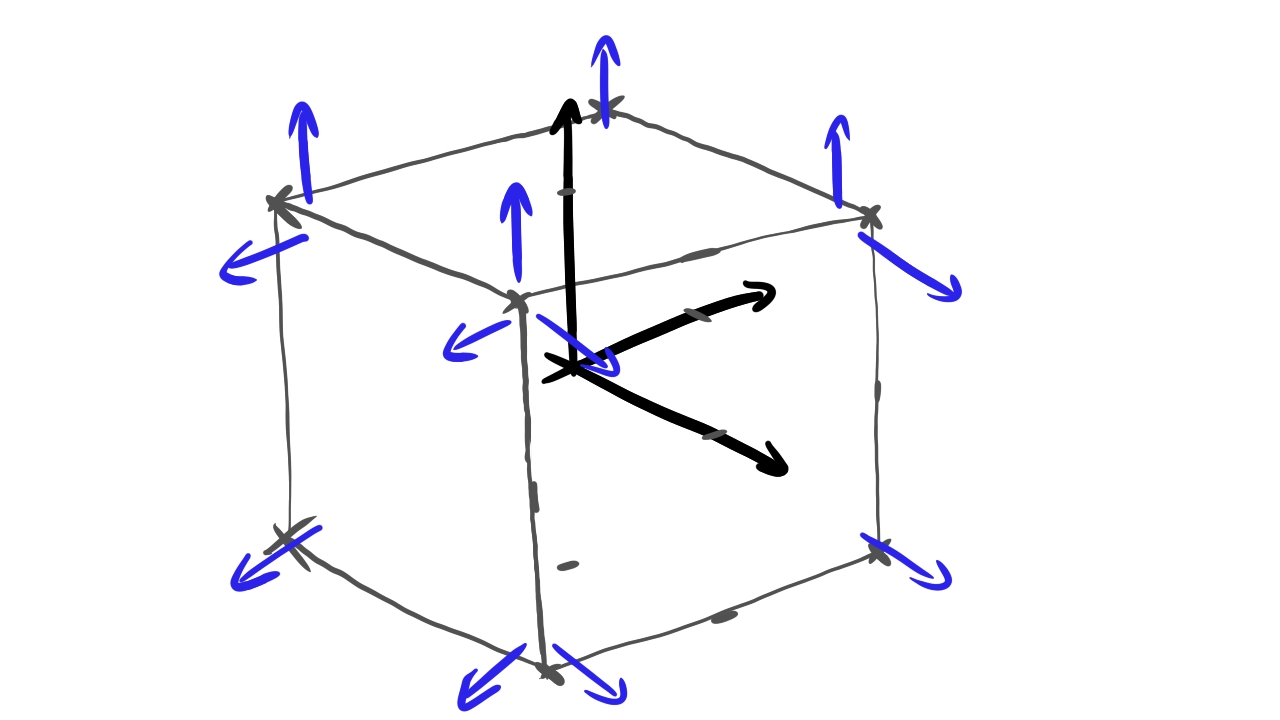
**Figure 10:** Illustration of the cube normals. The cube normals will point outwards, the positive z face's normal will point to the positive z direction, the negative y's will point to the negative y direction, and so on. When shaded, every cube face will look flat, with sudden changes along the axes.

The new content of the array will be the following:


    vec![
        // Pos Z
        //   Vertex 0
        -0.5, -0.5, 0.5,
        //   Normal 0
        0.0, 0.0, 1.0,
        //   TexCoord 0
        0.0, 0.0,
        //   Vertex 1
        -0.5, 0.5, 0.5,
        //   Normal 1
        0.0, 0.0, 1.0,
        //   TexCoord 1
        0.0, 1.0,
        //   Vertex 2
        0.5, 0.5, 0.5,
        //   Normal 2
        0.0, 0.0, 1.0,
        //   TexCoord 2
        1.0, 1.0,
        //   Vertex 3
        0.5, -0.5, 0.5,
        //   Normal 3
        0.0, 0.0, 1.0,
        //   TexCoord 3
        1.0, 0.0,
        // Neg Z
        //   Vertex 0
        -0.5, -0.5, -0.5,
        //   Normal 0
        0.0, 0.0, -1.0,
        //   TexCoord 0
        0.0, 0.0,
        //   Vertex 1
        -0.5, 0.5, -0.5,
        //   Normal 1
        0.0, 0.0, -1.0,
        //   TexCoord 1
        0.0, 1.0,
        //   Vertex 2
        0.5, 0.5, -0.5,
        //   Normal 2
        0.0, 0.0, -1.0,
        //   TexCoord 2
        1.0, 1.0,
        //   Vertex 3
        0.5, -0.5, -0.5,
        //   Normal 3
        0.0, 0.0, -1.0,
        //   TexCoord 3
        1.0, 0.0,
        // Pos X
        //   Vertex 0
        0.5, -0.5, -0.5,
        //   Normal 0
        1.0, 0.0, 0.0,
        //   TexCoord 0
        0.0, 0.0,
        //   Vertex 1
        0.5, -0.5, 0.5,
        //   Normal 1
        1.0, 0.0, 0.0,
        //   TexCoord 1
        0.0, 1.0,
        //   Vertex 2
        0.5, 0.5, 0.5,
        //   Normal 2
        1.0, 0.0, 0.0,
        //   TexCoord 2
        1.0, 1.0,
        //   Vertex 3
        0.5, 0.5, -0.5,
        //   Normal 3
        1.0, 0.0, 0.0,
        //   TexCoord 3
        1.0, 0.0,
        // Neg X
        //   Vertex 0
        -0.5, -0.5, -0.5,
        //   Normal 0
        -1.0, 0.0, 0.0,
        //   TexCoord 0
        0.0, 0.0,
        //   Vertex 1
        -0.5, -0.5, 0.5,
        //   Normal 1
        -1.0, 0.0, 0.0,
        //   TexCoord 1
        0.0, 1.0,
        //   Vertex 2
        -0.5, 0.5, 0.5,
        //   Normal 2
        -1.0, 0.0, 0.0,
        //   TexCoord 2
        1.0, 1.0,
        //   Vertex 3
        -0.5, 0.5, -0.5,
        //   Normal 3
        -1.0, 0.0, 0.0,
        //   TexCoord 3
        1.0, 0.0,
        // Pos Y
        //   Vertex 0
        -0.5, 0.5, -0.5,
        //   Normal 0
        0.0, 1.0, 0.0,
        //   TexCoord 0
        0.0, 0.0,
        //   Vertex 1
        -0.5, 0.5, 0.5,
        //   Normal 1
        0.0, 1.0, 0.0,
        //   TexCoord 1
        0.0, 1.0,
        //   Vertex 2
        0.5, 0.5, 0.5,
        //   Normal 2
        0.0, 1.0, 0.0,
        //   TexCoord 2
        1.0, 1.0,
        //   Vertex 3
        0.5, 0.5, -0.5,
        //   Normal 3
        0.0, 1.0, 0.0,
        //   TexCoord 3
        1.0, 0.0,
        // Neg Y
        //   Vertex 0
        -0.5, -0.5, -0.5,
        //   Normal 0
        0.0, -1.0, 0.0,
        //   TexCoord 0
        0.0, 0.0,
        //   Vertex 1
        -0.5, -0.5, 0.5,
        //   Normal 1
        0.0, -1.0, 0.0,
        //   TexCoord 1
        0.0, 1.0,
        //   Vertex 2
        0.5, -0.5, 0.5,
        //   Normal 2
        0.0, -1.0, 0.0,
        //   TexCoord 2
        1.0, 1.0,
        //   Vertex 3
        0.5, -0.5, -0.5,
        //   Normal 3
        0.0, -1.0, 0.0,
        //   TexCoord 3
        1.0, 0.0,
    ]

Setting up the graphics pipeline

Now that we have set up the data for the normal vectors in the CPU side vertex data, it will be uploaded automatically, and the buffers will be sized correctly, but the shader needs to access the new data, just as it did with the texture coordinates.

For that we need to add the normal as a vertex attribute, just as we did with the texture coordinates.


    //
    // Pipeline state
    //

    // ...

    let vertex_bindings = [
        VkVertexInputBindingDescription {
            binding: 0,
            stride: 8 * core::mem::size_of::<f32>() as u32,
            inputRate: VK_VERTEX_INPUT_RATE_VERTEX,
        }
    ];

    let vertex_attributes = [
        VkVertexInputAttributeDescription {
            location: 0,
            binding: 0,
            format: VK_FORMAT_R32G32B32_SFLOAT,
            offset: 0,
        },
        VkVertexInputAttributeDescription {
            location: 1,
            binding: 0,
            format: VK_FORMAT_R32G32B32_SFLOAT,
            offset: 3 * core::mem::size_of::<f32>() as u32,
        },
        VkVertexInputAttributeDescription {
            location: 2,
            binding: 0,
            format: VK_FORMAT_R32G32_SFLOAT,
            offset: 6 * core::mem::size_of::<f32>() as u32,
        }
    ];

    let vertex_input_state = VkPipelineVertexInputStateCreateInfo {
        sType: VK_STRUCTURE_TYPE_PIPELINE_VERTEX_INPUT_STATE_CREATE_INFO,
        pNext: core::ptr::null(),
        flags: 0x0,
        vertexBindingDescriptionCount: vertex_bindings.len() as u32,
        pVertexBindingDescriptions: vertex_bindings.as_ptr(),
        vertexAttributeDescriptionCount: vertex_attributes.len() as u32,
        pVertexAttributeDescriptions: vertex_attributes.as_ptr()
    };

    // ...

Pay attention that we reorganized our attributes a bit, now location 1 will belong to the normal, and the texture coordinates are moved to location 2.

The stride has also changed! We needed to add 3 floats per vertex to represent normals, and this needs to be reflected here. Previously it was 5 floats but now it's 8!

We calculate indexed draw call offsets using this stride where we define the draw call parameters of our models, so we need to update it there as well.



    //
    // Model and Texture ID-s
    //

    // ...

    const PER_VERTEX_DATA_SIZE: usize = 8;

    // ...

Now the draw call params for our models will be calculated correctly.

Adding material data and light array

The specialized version of the rendering equation requires material and light data, and if we want to run it on the GPU, then the GPU-side scene representation will need to store this new data. We will need to upload material and light data into uniform buffer regions. The material data will be placed in a tightly packed array separate from the transforms, because the fragment shader only needs the material data, and interleaving it with the transform data would be a waste of memory bandwidth. The light data will be stored in a third tightly packed array. We also need to upload a new variable for the exposure value.

To summarize, we will have the following uniform buffer regions:

the transform array containing the camera data at the beginning and the model matrix array after
the material array containing the exposure value at the beginning and the material data array after
the light array containing the light count and the light data array

Let's start writing the code that defines our data structures!

UBO layout

First we look at the vertex shader UBO layout. We want a single per scene camera data and an array of model matrices. The data structure from the previous tutorials will work fine, so we leave the memory layout unchanged. We just rename ObjectData to TransformData, because now it only contains a piece of the "object data", the object transform. The other piece is the material data, which will be in a different array accessible to the fragment shader. Now that the "object data" is split in two, a more specific name is more fitting.

For the sake of completeness the shader code is the following:


struct CameraData
{
    mat4 projection_matrix;
    mat4 view_matrix;
};

struct TransformData
{
    mat4 model_matrix;
};

const uint MAX_UBO_DESCRIPTOR_COUNT = 8;
const uint MAX_OBJECT_COUNT = 64;

layout(std140, set=0, binding = 0) uniform UniformData {
    CameraData cam_data;
    TransformData transform_data[MAX_OBJECT_COUNT];
} uniform_transform_data[MAX_UBO_DESCRIPTOR_COUNT];

The renamed Rust struct matching the transform data is the following:


    //
    // Uniform data
    //

    // ...

    #[repr(C, align(16))]
    #[derive(Copy, Clone)]
    struct TransformData
    {
        model_matrix: [f32; 16]
    }

    // ...

Then we define the structs of the material region as well, which will contain the per scene exposure settings and the per object material data. We create the data structures ExposureData and MaterialData.

The shader code defining the material data is the following:


const uint MAX_UBO_DESCRIPTOR_COUNT = 8;
const uint MAX_OBJECT_COUNT = 64;

struct MaterialData
{
    vec4 albedo;
    vec4 emissive;
};

layout(std140, set=0, binding = 2) uniform UniformMaterialData {
    float exposure_value;
    MaterialData material_data[MAX_OBJECT_COUNT];
} uniform_material_data[MAX_UBO_DESCRIPTOR_COUNT];

The matching Rust structs are the following:


    //
    // Uniform data
    //

    // ...

    #[repr(C, align(16))]
    #[derive(Copy, Clone)]
    struct ExposureData
    {
        exposure_value: f32,
        std140_padding_0: f32,
        std140_padding_1: f32,
        std140_padding_2: f32
    }

    #[repr(C, align(16))]
    #[derive(Copy, Clone)]
    struct MaterialData
    {
        albedo: [f32; 4],
        emissive: [f32; 4]
    }

    // ...

The last region will be the light data where the per scene light count will be stored at the beginning, and per light data for every light after. We create the data structures LightCountData and LightData.

The shader code for the light array is the following:


const uint MAX_UBO_DESCRIPTOR_COUNT = 8;
const uint MAX_LIGHT_COUNT = 64;

struct LightData
{
    vec4 position;
    vec4 intensity;
};

layout(std140, set=0, binding = 3) uniform UniformLightData {
    uint light_count;
    LightData light_data[MAX_LIGHT_COUNT];
} uniform_light_data[MAX_UBO_DESCRIPTOR_COUNT];

The matching Rust structs are the following:


    //
    // Uniform data
    //

    // ...

    #[repr(C, align(16))]
    #[derive(Copy, Clone)]
    struct LightCountData
    {
        light_count: u32,
        std140_padding_0: f32,
        std140_padding_1: f32,
        std140_padding_2: f32,
    }

    #[repr(C, align(16))]
    #[derive(Copy, Clone)]
    struct LightData
    {
        position: [f32; 4],
        intensity: [f32; 4]
    }

    // ...

Now that our data structures are defined properly, we need to size our buffer in a way that all three buffer range fits into it, and can be accessed using UBO offsets. Offsets have alignment requirements: they must be aligned to minUniformBufferOffsetAlignment. This means that we need to pad our uniform buffer regions to make sure regions laid out one after another begin on an offset that is an integer multiple of minUniformBufferOffsetAlignment.


    //
    // Uniform data
    //

    // ...

    let min_ubo_offset_alignment = phys_device_properties.limits.minUniformBufferOffsetAlignment as usize;

    let max_object_count = 64;

    // Per frame UBO transform region size

    let transform_data_size = core::mem::size_of::<CameraData>() + max_object_count * core::mem::size_of::<TransformData>();

    let transform_data_align_rem = transform_data_size % min_ubo_offset_alignment;
    let transform_data_padding;
    if transform_data_align_rem != 0
    {
        transform_data_padding = min_ubo_offset_alignment - transform_data_align_rem;
    }
    else
    {
        transform_data_padding = 0;
    }

    let padded_transform_data_size = transform_data_size + transform_data_padding;

First we determine the higher bound to the amount of scene elements to render, max_object_count, which will be 64.

Then we start figuring out the transform region size for a single frame. The useful data will need core::mem::size_of::<CameraData>() amount of space to store the camera data, and max_object_count * core::mem::size_of::<TransformData>() amount of space to store the transforms for every scene object. Since these structs are padded according to the std140 alignment rules, their simple sum will yield the amount of space the useful data will require.

Then we need to see if the resulting size will satisfy the alignment requirements. We take the remainder with the required offset alignment, and if it's not zero, then we add enough bytes to round the region size to an integer multiple of the required offset alignment.


    // Per frame UBO material region size

    let material_data_size = core::mem::size_of::<ExposureData>() + max_object_count * core::mem::size_of::<MaterialData>();

    let material_data_align_rem = material_data_size % min_ubo_offset_alignment;
    let material_data_padding;
    if material_data_align_rem != 0
    {
        material_data_padding = min_ubo_offset_alignment - material_data_align_rem;
    }
    else
    {
        material_data_padding = 0;
    }

    let padded_material_data_size = material_data_size + material_data_padding;

Calculating the material data size for a single frame follows the same principles, only this time the struct sizes are core::mem::size_of::<ExposureData>() and core::mem::size_of::<MaterialData>().


    let max_light_count = 64;

    // Per frame UBO light region size

    let light_data_size = core::mem::size_of::<LightCountData>() + max_light_count * core::mem::size_of::<LightData>();

    let light_data_align_rem = light_data_size % min_ubo_offset_alignment;
    let light_data_padding;
    if light_data_align_rem != 0
    {
        light_data_padding = min_ubo_offset_alignment - light_data_align_rem;
    }
    else
    {
        light_data_padding = 0;
    }

    let padded_light_data_size = light_data_size + light_data_padding;

The same goes for the light region for a single frame, this time with the struct sizes core::mem::size_of::<LightCountData>() and core::mem::size_of::<LightData>().


    // Total UBO size

    let total_transform_data_size = frame_count * padded_transform_data_size;
    let total_material_data_size = frame_count * padded_material_data_size;
    let total_light_data_size = frame_count * padded_light_data_size;
    let uniform_buffer_size = total_transform_data_size + total_material_data_size + total_light_data_size;

    // ...

Finally we need to figure out the memory requirements for every frame. First let's specify the memory arrangement! First we place the transform regions for every frame one after the other. Then the material data regions for every frame one after the other, and finally the light regions one after the other.

The memory requirements for the transform regions laid out like this is frame_count * padded_transform_data_size, and the other regions are analogous. Then we sum up all of the regions to get the total uniform buffer size.

Now it's time to update the descriptor set layout.

Setting up descriptor set layout

We want to access two new uniform buffer regions per frame, and this will require new uniform buffer bindings. We start with adding these to the descriptor set layout.


    //
    // Descriptor set layout
    //

    // ...

    let layout_bindings = [
        VkDescriptorSetLayoutBinding {
            binding: 0,
            descriptorType: VK_DESCRIPTOR_TYPE_UNIFORM_BUFFER,
            descriptorCount: max_ubo_descriptor_count,
            stageFlags: VK_SHADER_STAGE_VERTEX_BIT as VkShaderStageFlags,
            pImmutableSamplers: core::ptr::null()
        },
        VkDescriptorSetLayoutBinding {
            binding: 1,
            descriptorType: VK_DESCRIPTOR_TYPE_COMBINED_IMAGE_SAMPLER,
            descriptorCount: max_tex2d_descriptor_count,
            stageFlags: VK_SHADER_STAGE_FRAGMENT_BIT as VkShaderStageFlags,
            pImmutableSamplers: core::ptr::null()
        },
        VkDescriptorSetLayoutBinding {
            binding: 2,
            descriptorType: VK_DESCRIPTOR_TYPE_UNIFORM_BUFFER,
            descriptorCount: max_ubo_descriptor_count,
            stageFlags: VK_SHADER_STAGE_FRAGMENT_BIT as VkShaderStageFlags,
            pImmutableSamplers: core::ptr::null()
        },
        VkDescriptorSetLayoutBinding {
            binding: 3,
            descriptorType: VK_DESCRIPTOR_TYPE_UNIFORM_BUFFER,
            descriptorCount: max_ubo_descriptor_count,
            stageFlags: VK_SHADER_STAGE_FRAGMENT_BIT as VkShaderStageFlags,
            pImmutableSamplers: core::ptr::null()
        }
    ];

    // ...

We append two new uniform buffer bindings, binding 2 and 3. These will be available from the VK_SHADER_STAGE_FRAGMENT_BIT, and will contain max_ubo_descriptor_count descriptors, following the descriptor array scheme first introduced in the uniform buffer chapter.

Setting up pipeline layout

We will have two new uniform buffer bindings to the fragment shader, the material and light data regions. They will be descriptor arrays, one descriptor per frame, and the material data region contains an array with per scene object data. To index into these arrays, we will need the push constants previously only available in the vertex shader, so we need to adjust our push constant ranges.


    //
    // Pipeline layout
    //

    // ...

    // Object ID + Frame ID
    let vertex_push_constant_size = 2 * core::mem::size_of::<u32>() as u32;
    // Object ID + Frame ID + Texture ID
    let fragment_push_constant_size = 3 * core::mem::size_of::<u32>() as u32;

    let push_constant_ranges = [
        VkPushConstantRange {
            stageFlags: VK_SHADER_STAGE_VERTEX_BIT as VkShaderStageFlags,
            offset: 0,
            size: vertex_push_constant_size,
        },
        VkPushConstantRange {
            stageFlags: VK_SHADER_STAGE_FRAGMENT_BIT as VkShaderStageFlags,
            offset: 0,
            size: fragment_push_constant_size,
        }
    ];

    // ...

The fragment shader's push constant range now spans three integers, the object index, the frame index and the texture index, and starts at zero offset.

Setting up descriptor pool and descriptor set

Now it's time to update everything related to descriptor set pools and descriptor sets, including writing the descriptor sets.

First let's update the descriptor pool sizes! We added two new bindings, each containing max_ubo_descriptor_count descriptors. That means we need three times the amount of uniform buffer descriptors as before, so let's adjust those pool sizes!


    //
    // Descriptor pool & descriptor set
    //

    let pool_sizes = [
        VkDescriptorPoolSize {
            type_: VK_DESCRIPTOR_TYPE_UNIFORM_BUFFER,
            descriptorCount: max_ubo_descriptor_count * 3
        },
        VkDescriptorPoolSize {
            type_: VK_DESCRIPTOR_TYPE_COMBINED_IMAGE_SAMPLER,
            descriptorCount: max_tex2d_descriptor_count
        }
    ];

    // ...

There. A factor of 3 in the uniform buffer pool size.

Now let's fill the descriptor set! This is one of the places where the decisions we made about the layout of uniform buffer regions start to matter, so pay attention! Here are the uniform buffer descriptor writes:


    //
    // Descriptor pool & descriptor set
    //

    // ...

    // Writing UBO descriptors

    let mut transform_ubo_descriptor_writes = Vec::with_capacity(max_ubo_descriptor_count as usize);
    for i in 0..max_ubo_descriptor_count
    {
        let ubo_region_index = (frame_count - 1).min(i as usize);
        transform_ubo_descriptor_writes.push(
            VkDescriptorBufferInfo {
                buffer: uniform_buffer,
                offset: (
                    ubo_region_index * padded_transform_data_size
                ) as VkDeviceSize,
                range: transform_data_size as VkDeviceSize
            }
        );
    }

    let mut material_ubo_descriptor_writes = Vec::with_capacity(max_ubo_descriptor_count as usize);
    for i in 0..max_ubo_descriptor_count
    {
        let ubo_region_index = (frame_count - 1).min(i as usize);
        material_ubo_descriptor_writes.push(
            VkDescriptorBufferInfo {
                buffer: uniform_buffer,
                offset: (
                    total_transform_data_size +
                    ubo_region_index * padded_material_data_size
                ) as VkDeviceSize,
                range: material_data_size as VkDeviceSize
            }
        );
    }

    let mut light_ubo_descriptor_writes = Vec::with_capacity(max_ubo_descriptor_count as usize);
    for i in 0..max_ubo_descriptor_count
    {
        let ubo_region_index = (frame_count - 1).min(i as usize);
        light_ubo_descriptor_writes.push(
            VkDescriptorBufferInfo {
                buffer: uniform_buffer,
                offset: (
                    total_transform_data_size + total_material_data_size +
                    ubo_region_index * padded_light_data_size
                ) as VkDeviceSize,
                range: light_data_size as VkDeviceSize
            }
        );
    }

    // ...

First we prepare the transform data descriptor writes. The first transform data region resides at the beginning of the uniform buffer, and the rest of the regions are laid out one after the other. The first loop fills the transform descriptor writes with the offsets starting at the beginning of the buffer, and in every iteration the offset is bumped by padded_transform_data_size for every region.

Then we prepare material data descriptor writes. The material data regions reside after the transform regions, so the offset of the material regions start at total_transform_data_size and the offsets are bumped by padded_material_data_size.

Finally we fill the light data descriptor writes. They come after the material data regions, so the offset of the light regions start at total_transform_data_size + total_material_data_size, and in every iteration the offset increases by padded_light_data_size.

Now that we prepared the descriptor writes, it's time to issue them.


    //
    // Descriptor pool & descriptor set
    //

    // ...

    let descriptor_set_writes = [
        VkWriteDescriptorSet {
            sType: VK_STRUCTURE_TYPE_WRITE_DESCRIPTOR_SET,
            pNext: core::ptr::null(),
            dstSet: descriptor_set,
            dstBinding: 0,
            dstArrayElement: 0,
            descriptorCount: transform_ubo_descriptor_writes.len() as u32,
            descriptorType: VK_DESCRIPTOR_TYPE_UNIFORM_BUFFER,
            pImageInfo: core::ptr::null(),
            pBufferInfo: transform_ubo_descriptor_writes.as_ptr(),
            pTexelBufferView: core::ptr::null()
        },
        VkWriteDescriptorSet {
            sType: VK_STRUCTURE_TYPE_WRITE_DESCRIPTOR_SET,
            pNext: core::ptr::null(),
            dstSet: descriptor_set,
            dstBinding: 1,
            dstArrayElement: 0,
            descriptorCount: tex2d_descriptor_writes.len() as u32,
            descriptorType: VK_DESCRIPTOR_TYPE_COMBINED_IMAGE_SAMPLER,
            pImageInfo: tex2d_descriptor_writes.as_ptr(),
            pBufferInfo: core::ptr::null(),
            pTexelBufferView: core::ptr::null()
        },
        VkWriteDescriptorSet {
            sType: VK_STRUCTURE_TYPE_WRITE_DESCRIPTOR_SET,
            pNext: core::ptr::null(),
            dstSet: descriptor_set,
            dstBinding: 2,
            dstArrayElement: 0,
            descriptorCount: material_ubo_descriptor_writes.len() as u32,
            descriptorType: VK_DESCRIPTOR_TYPE_UNIFORM_BUFFER,
            pImageInfo: core::ptr::null(),
            pBufferInfo: material_ubo_descriptor_writes.as_ptr(),
            pTexelBufferView: core::ptr::null()
        },
        VkWriteDescriptorSet {
            sType: VK_STRUCTURE_TYPE_WRITE_DESCRIPTOR_SET,
            pNext: core::ptr::null(),
            dstSet: descriptor_set,
            dstBinding: 3,
            dstArrayElement: 0,
            descriptorCount: light_ubo_descriptor_writes.len() as u32,
            descriptorType: VK_DESCRIPTOR_TYPE_UNIFORM_BUFFER,
            pImageInfo: core::ptr::null(),
            pBufferInfo: light_ubo_descriptor_writes.as_ptr(),
            pTexelBufferView: core::ptr::null()
        }
    ];

    // ...

We adjusted the previous tutorials' uniform upload struct for the transform data, adjusting it to take transform_ubo_descriptor_writes as a parameter, and we add two new descriptor writes, one taking light_ubo_descriptor_writes and another taking material_ubo_descriptor_writes as a parameter.

This takes care of the descriptor writes of the new uniform buffer regions.

CPU side scene representation

In the 3D tutorial we have created a StaticMesh struct which maintained the scene's CPU side state. Previously it only contained transform data. Now that the rendering equation requires additional data, we must extend our StaticMesh data structure to contain material data. We need to add the constant parameters for the diffuse BRDF and the emissive lighting, so let's add those new fields!


    //
    // Game state
    //

    // ...

    // Game logic state

    // ...

    struct StaticMesh
    {
        x: f32,
        y: f32,
        z: f32,
        scale: f32,
        rot_x: f32,
        rot_y: f32,
        albedo_r: f32,
        albedo_g: f32,
        albedo_b: f32,
        emissive_r: f32,
        emissive_g: f32,
        emissive_b: f32,
        texture_index: u32,
        model_index: usize
    }

    // ...

We added three new albedo fields, one for each color channel, which will contain the diffuse BRDF parameters for each corresponding wavelength. We also added three emissive fields, one for each color channel, which will contain the emitted radiance for each color channel.

The rendering equation also requires lights, so we add a whole new type of scene elements, lights. We need to store their position and radiant intensity for every wavelength.


    //
    // Game state
    //

    // ...

    // Game logic state

    // ...

    struct Light
    {
        x: f32,
        y: f32,
        z: f32,
        intensity_r: f32,
        intensity_g: f32,
        intensity_b: f32
    }

    // ...

We have created our new struct, Light, and it has the x, y and z fields to store the position, and the intensity fields to store the radiant intensity for every color channel.

Now that we have updated our scene data structures, let's fill the new fields for our scene elements.

First let's add a float for exposure correction! We will use this as exposure value during the exposure correction step, and we will be able to adjust it using the keyboard.


    //
    // Game state
    //

    // ...

    // Game logic state

    // ...

    let mut exposure_value = 9.0;

    // ...

Our variable will be exposure_value and by default we set it to 9.0, which is a value I stole from wikipedia. There is a table of exposure values for various lighting conditions, and 9 is the value for Neon and other bright signs. The scene I am about to include will look fine with this default exposure value, but we will increase and decrease it using the keyboard later.

As for the scene objects, we need to add material data. For the sake of simplicity, I'm just inlining the whole scene right here instead of only including the material data. It's simpler to copy paste this way.


    //
    // Game state
    //

    // ...

    // Game logic state

    // ...

    let player_id = 0;

    let mut static_meshes = Vec::with_capacity(max_object_count);
    static_meshes.push(
        StaticMesh {
            x: 0.25,
            y: 0.0,
            z: -1.25,
            scale: 0.25,
            rot_x: 0.0,
            rot_y: 0.0,
            albedo_r: 1.0,
            albedo_g: 1.0,
            albedo_b: 1.0,
            emissive_r: 0.0,
            emissive_g: 0.0,
            emissive_b: 0.0,
            texture_index: red_yellow_green_black_tex_index,
            model_index: triangle_index
        }
    );
    static_meshes.push(
        StaticMesh {
            x: 0.25,
            y: -0.25,
            z: -2.0,
            scale: 0.25,
            rot_x: 0.0,
            rot_y: 0.0,
            albedo_r: 0.75,
            albedo_g: 0.5,
            albedo_b: 1.0,
            emissive_r: 0.0,
            emissive_g: 0.0,
            emissive_b: 0.0,
            texture_index: blue_cyan_magenta_white_tex_index,
            model_index: triangle_index
        }
    );
    static_meshes.push(
        StaticMesh {
            x: -0.25,
            y: 0.25,
            z: -3.0,
            scale: 0.25,
            rot_x: 0.0,
            rot_y: 0.0,
            albedo_r: 0.75,
            albedo_g: 0.5,
            albedo_b: 1.0,
            emissive_r: 0.0,
            emissive_g: 0.0,
            emissive_b: 0.0,
            texture_index: blue_cyan_magenta_white_tex_index,
            model_index: quad_index
        }
    );
    static_meshes.push(
        StaticMesh {
            x: 1.5,
            y: 0.0,
            z: -2.6,
            scale: 0.25,
            rot_x: 0.0,
            rot_y: 0.0,
            albedo_r: 1.0,
            albedo_g: 1.0,
            albedo_b: 1.0,
            emissive_r: 0.0,
            emissive_g: 0.0,
            emissive_b: 0.0,
            texture_index: red_yellow_green_black_tex_index,
            model_index: quad_index
        }
    );
    static_meshes.push(
        StaticMesh {
            x: -1.5,
            y: 0.0,
            z: -2.6,
            scale: 0.25,
            rot_x: 0.0,
            rot_y: 0.0,
            albedo_r: 1.0,
            albedo_g: 1.0,
            albedo_b: 1.0,
            emissive_r: 0.0,
            emissive_g: 0.0,
            emissive_b: 0.0,
            texture_index: blue_cyan_magenta_white_tex_index,
            model_index: quad_index
        }
    );

    // Cubes added later

    static_meshes.push(
        StaticMesh {
            x: 1.0,
            y: 0.5,
            z: -2.5,
            scale: 0.25,
            rot_x: 0.0,
            rot_y: 0.0,
            albedo_r: 1.0,
            albedo_g: 1.0,
            albedo_b: 1.0,
            emissive_r: 0.0,
            emissive_g: 0.0,
            emissive_b: 0.0,
            texture_index: red_yellow_green_black_tex_index,
            model_index: cube_index
        }
    );
    static_meshes.push(
        StaticMesh {
            x: 1.0,
            y: -0.5,
            z: -2.5,
            scale: 0.25,
            rot_x: 0.0,
            rot_y: 0.0,
            albedo_r: 1.0,
            albedo_g: 1.0,
            albedo_b: 1.0,
            emissive_r: 0.0,
            emissive_g: 0.0,
            emissive_b: 0.0,
            texture_index: red_yellow_green_black_tex_index,
            model_index: cube_index
        }
    );
    static_meshes.push(
        StaticMesh {
            x: -1.0,
            y: 0.5,
            z: -2.5,
            scale: 0.25,
            rot_x: 0.0,
            rot_y: 0.0,
            albedo_r: 1.0,
            albedo_g: 1.0,
            albedo_b: 1.0,
            emissive_r: 0.0,
            emissive_g: 0.0,
            emissive_b: 0.0,
            texture_index: blue_cyan_magenta_white_tex_index,
            model_index: cube_index
        }
    );
    static_meshes.push(
        StaticMesh {
            x: -1.0,
            y: -0.5,
            z: -2.5,
            scale: 0.25,
            rot_x: 0.0,
            rot_y: 0.0,
            albedo_r: 1.0,
            albedo_g: 1.0,
            albedo_b: 1.0,
            emissive_r: 0.0,
            emissive_g: 0.0,
            emissive_b: 0.0,
            texture_index: blue_cyan_magenta_white_tex_index,
            model_index: cube_index
        }
    );

    // ...

These are the models from the previous tutorial with some material data assigned to them.

Finally we add lights. I will add the following light sources:


    //
    // Game state
    //

    // ...

    // Game logic state

    // ...

    let mut lights = Vec::with_capacity(max_light_count);
    lights.push(
        Light {
            x: 0.0,
            y: 0.0,
            z: 0.0,
            intensity_r: 0.5,
            intensity_g: 0.5,
            intensity_b: 0.5
        }
    );
    lights.push(
        Light {
            x: 0.25,
            y: -0.25,
            z: -1.9,
            intensity_r: 0.025,
            intensity_g: 0.025,
            intensity_b: 0.025
        }
    );
    lights.push(
        Light {
            x: -0.25,
            y: 0.25,
            z: -2.9,
            intensity_r: 0.025,
            intensity_g: 0.025,
            intensity_b: 0.025
        }
    );
    lights.push(
        Light {
            x: 1.5,
            y: 0.0,
            z: -2.5,
            intensity_r: 0.125,
            intensity_g: 0.125,
            intensity_b: 0.025
        }
    );
    lights.push(
        Light {
            x: -1.5,
            y: 0.0,
            z: -2.5,
            intensity_r: 0.125,
            intensity_g: 0.025,
            intensity_b: 0.025
        }
    );
    lights.push(
        Light {
            x: -1.0,
            y: 0.0,
            z: -2.9,
            intensity_r: 0.25,
            intensity_g: 0.25,
            intensity_b: 0.25
        }
    );
    lights.push(
        Light {
            x: 1.0,
            y: 0.0,
            z: -2.9,
            intensity_r: 0.25,
            intensity_g: 0.25,
            intensity_b: 0.25
        }
    );

    // ...

Now that we have a basic game state, let's update our logic to update it using the keyboard!

Controlling exposure from keyboard

We want to control the exposure value using the keyboard. As with every other key from before, we need to remember if the key is pressed. For this we need a few new booleans.


    //
    // Game state
    //

    // Input state

    // ...

    let mut exposure_increase = false;
    let mut exposure_decrease = false;

The exposure_increase will contain whether we hold the button we assign to increasing the exposure value, and the exposure_decrease will contain whether we hold the decrease button.

Now let's update them when the right key events arrive!



    //
    // Game loop
    //

    // ...

    let mut event_pump = sdl.event_pump().unwrap();
    'main: loop
    {
        for event in event_pump.poll_iter()
        {
            match event
            {
                sdl2::event::Event::Quit { .. } =>
                {
                    break 'main;
                }
                sdl2::event::Event::Window { win_event, .. } =>
                {
                    // ...
                }
                sdl2::event::Event::KeyDown { keycode: Some(keycode), .. } =>
                {
                    // ...

                    if keycode == sdl2::keyboard::Keycode::Y
                    {
                        exposure_increase = true;
                    }
                    if keycode == sdl2::keyboard::Keycode::X
                    {
                        exposure_decrease = true;
                    }
                }
                sdl2::event::Event::KeyUp { keycode: Some(keycode), .. } =>
                {
                    // ...

                    if keycode == sdl2::keyboard::Keycode::Y
                    {
                        exposure_increase = false;
                    }
                    if keycode == sdl2::keyboard::Keycode::X
                    {
                        exposure_decrease = false;
                    }
                }
                _ =>
                {}
            }
        }

        // ...
    }

I assigned the Y button to increasing, and the X button to decreasing the exposure value. If you are using a non-QWERTZ keyboard, you probably want to assign it differently.

Now that we know whether the exposure increase or exposure decrease buttons are held, let's handle it in the game logic!


        //
        // Logic
        //

        // ...

        if exposure_increase
        {
            exposure_value += 0.1;
        }
        if exposure_decrease
        {
            exposure_value -= 0.1;
        }

If the exposure increase button is held, we add to the exposure value in every frame, and if the exposure decrease button is held, then we subtract from it.

Now it's time to upload our new data to the GPU.

Data upload

We have new uniform buffer regions to fill, and we have extended our game state to serve as a data source, so it's time to update our upload logic.

First let's create struct references and slices to the uniform buffer regions!


        //
        // Rendering
        //

        //
        // Uniform upload
        //

        {
            // Getting references

            let current_frame_transform_region_offset = (
                current_frame_index * padded_transform_data_size
            ) as isize;
            let camera_data;
            let transform_data_array;
            unsafe {
                let per_frame_transform_region_begin = uniform_buffer_ptr.offset(
                    current_frame_transform_region_offset
                );

                let camera_data_ptr: *mut core::mem::MaybeUninit<CameraData> = core::mem::transmute(
                    per_frame_transform_region_begin
                );
                camera_data = &mut *camera_data_ptr;

                let transform_offset = core::mem::size_of::<CameraData>() as isize;
                let transform_data_ptr: *mut core::mem::MaybeUninit<TransformData> = core::mem::transmute(
                    per_frame_transform_region_begin.offset(transform_offset)
                );
                transform_data_array = core::slice::from_raw_parts_mut(
                    transform_data_ptr,
                    max_object_count
                );
            }

            let current_frame_material_region_offset = (
                total_transform_data_size +
                current_frame_index * padded_material_data_size
                ) as isize;
            let exposure_data;
            let material_data_array;
            unsafe {
                let per_frame_material_region_begin = uniform_buffer_ptr.offset(
                    current_frame_material_region_offset
                );

                let exposure_data_ptr: *mut core::mem::MaybeUninit<ExposureData> = core::mem::transmute(
                    per_frame_material_region_begin
                );
                exposure_data = &mut *exposure_data_ptr;

                let material_offset = core::mem::size_of::<ExposureData>() as isize;
                let material_data_ptr: *mut core::mem::MaybeUninit<MaterialData> = core::mem::transmute(
                    per_frame_material_region_begin.offset(material_offset)
                );
                material_data_array = core::slice::from_raw_parts_mut(
                    material_data_ptr,
                    max_object_count
                );
            }

            let current_frame_light_region_offset = (
                total_transform_data_size + total_material_data_size +
                current_frame_index * padded_light_data_size
            ) as isize;
            let light_count_data;
            let light_data_array;
            unsafe {
                let per_frame_light_region_begin = uniform_buffer_ptr.offset(
                    current_frame_light_region_offset
                );

                let light_count_data_ptr: *mut core::mem::MaybeUninit<LightCountData> = core::mem::transmute(
                    per_frame_light_region_begin
                );
                light_count_data = &mut *light_count_data_ptr;

                let light_offset = core::mem::size_of::<LightCountData>() as isize;
                let light_data_ptr: *mut core::mem::MaybeUninit<LightData> = core::mem::transmute(
                    per_frame_light_region_begin.offset(light_offset)
                );
                light_data_array = core::slice::from_raw_parts_mut(
                    light_data_ptr,
                    max_light_count
                );
            }

            // ...
        }

        // ...

For every region we need to find the offset first. Pay attention that this follows the formulae we used during the descriptor writes. The transform regions lie at the beginning of the uniform buffer, so the region of the current frame is just current_frame_index * padded_transform_data_size. The material regions lie after all the transform regions, so the material region of the current frame is at the offset total_transform_data_size + current_frame_index * padded_material_data_size. Finally the lights lie after all the material arrays, so their offset is at total_transform_data_size + total_material_data_size + current_frame_index * padded_light_data_size.

Once we have the region offset, turning it into struct references and slices follows the same principles as the previous tutorials, only we have more of them.

Now let's adjust our existing upload logic! We have a new name for our transform array, and we need to update the transform upload accordingly.


        //
        // Rendering
        //

        //
        // Uniform upload
        //

        {
            // Getting references

            // ...

            // Filling them with data

            let field_of_view_angle = core::f32::consts::PI / 3.0;
            let aspect_ratio = width as f32 / height as f32;
            let far = 100.0;
            let near = 0.1;
            let projection_matrix = perspective(
                field_of_view_angle,
                aspect_ratio,
                far,
                near
            );

            *camera_data = core::mem::MaybeUninit::new(
                CameraData {
                    projection_matrix: mat_mlt(
                        &projection_matrix,
                        &scale(1.0, -1.0, -1.0)
                    ),
                    view_matrix: mat_mlt(
                        &rotate_x(-camera.rot_x),
                        &mat_mlt(
                            &rotate_y(-camera.rot_y),
                            &translate(
                                -camera.x,
                                -camera.y,
                                -camera.z
                            )
                        )
                    )
                }
            );

            let static_mesh_transform_data_array = &mut transform_data_array[..static_meshes.len()];
            for (i, static_mesh) in static_meshes.iter().enumerate()
            {
                static_mesh_transform_data_array[i] = core::mem::MaybeUninit::new(
                    TransformData {
                        model_matrix: mat_mlt(
                            &translate(
                                static_mesh.x,
                                static_mesh.y,
                                static_mesh.z
                            ),
                            &mat_mlt(
                                &rotate_x(static_mesh.rot_x),
                                &mat_mlt(
                                    &rotate_y(static_mesh.rot_y),
                                    &scale(
                                        static_mesh.scale,
                                        static_mesh.scale,
                                        static_mesh.scale
                                    )
                                )
                            )
                        )
                    }
                );
            }

            // ...
        }

        // ...

Instead of writing to the original object_data_array variable, we write to the new transform_data_array, and we use the new struct name TransformData.

Now we start writing new upload code. We need to upload the new material data!


        //
        // Rendering
        //

        //
        // Uniform upload
        //

        {
            // Getting references

            // ...

            // Filling them with data

            // ...

            *exposure_data = core::mem::MaybeUninit::new(
                ExposureData {
                    exposure_value: exposure_value,
                    std140_padding_0: 0.0,
                    std140_padding_1: 0.0,
                    std140_padding_2: 0.0
                }
            );

            let static_mesh_material_data_array = &mut material_data_array[..static_meshes.len()];
            for (i, static_mesh) in static_meshes.iter().enumerate()
            {
                static_mesh_material_data_array[i] = core::mem::MaybeUninit::new(
                    MaterialData {
                        albedo: [
                            static_mesh.albedo_r,
                            static_mesh.albedo_g,
                            static_mesh.albedo_b,
                            0.0
                        ],
                        emissive: [
                            static_mesh.emissive_r,
                            static_mesh.emissive_g,
                            static_mesh.emissive_b,
                            0.0
                        ]
                    }
                );
            }

            // ...
        }

        // ...

First we write the struct containing the exposure value to the beginning of the buffer region, then we iterate over every scene object and write their material data to the material_data_array.

Finally we need to upload our light data.


        //
        // Rendering
        //

        //
        // Uniform upload
        //

        {
            // Getting references

            // ...

            // Filling them with data

            // ...

            *light_count_data = core::mem::MaybeUninit::new(
                LightCountData {
                    light_count: lights.len() as u32,
                    std140_padding_0: 0.0,
                    std140_padding_1: 0.0,
                    std140_padding_2: 0.0
                }
            );

            for (i, light) in lights.iter().enumerate()
            {
                light_data_array[i] = core::mem::MaybeUninit::new(
                    LightData {
                        position: [
                            light.x,
                            light.y,
                            light.z,
                            0.0
                        ],
                        intensity: [
                            light.intensity_r,
                            light.intensity_g,
                            light.intensity_b,
                            0.0
                        ]
                    }
                );
            }
        }

        // ...

First we write the struct containing the light count to the light buffer region, then we iterate over every light and write their data into the light array.

Finally we have finished writing the uniform buffer upload. Now it's time to adjust command buffer recording!

Encoding command buffers

One of the first things we need to do is adjust the push constant upload. Previously the frame index and the object index were only used in the vertex shader, but we have adjusted the push constant ranges in the pipeline layout, and we will need them in the fragment shader. We will need the frame index to access the right material and light region, and we will need the object index to access the right material data, so let's add a few stage bits!


        //
        // Rendering commands
        //

        // ...

        unsafe
        {
            vkCmdBeginRenderPass(
                cmd_buffers[current_frame_index],
                &render_pass_begin_info,
                VK_SUBPASS_CONTENTS_INLINE
            );

            // ...

            // Setting per frame descriptor array index
            let ubo_desc_index: u32 = current_frame_index as u32;

            vkCmdPushConstants(
                cmd_buffers[current_frame_index],
                pipeline_layout,
                (VK_SHADER_STAGE_VERTEX_BIT | VK_SHADER_STAGE_FRAGMENT_BIT) as VkShaderStageFlags, // We changed this
                core::mem::size_of::<u32>() as u32,
                core::mem::size_of::<u32>() as u32,
                &ubo_desc_index as *const u32 as *const core::ffi::c_void
            );

            for (i, static_mesh) in static_meshes.iter().enumerate()
            {
                // Per obj array index
                let object_index = i as u32;

                vkCmdPushConstants(
                    cmd_buffers[current_frame_index],
                    pipeline_layout,
                    (VK_SHADER_STAGE_VERTEX_BIT | VK_SHADER_STAGE_FRAGMENT_BIT) as VkShaderStageFlags, // We changed this
                    0,
                    core::mem::size_of::<u32>() as u32,
                    &object_index as *const u32 as *const core::ffi::c_void
                );

                // Setting texture descriptor array index
                vkCmdPushConstants(
                    cmd_buffers[current_frame_index],
                    pipeline_layout,
                    VK_SHADER_STAGE_FRAGMENT_BIT as VkShaderStageFlags,
                    2 * core::mem::size_of::<u32>() as u32,
                    core::mem::size_of::<u32>() as u32,
                    &static_mesh.texture_index as *const u32 as *const core::ffi::c_void
                );

                vkCmdDrawIndexed(
                    cmd_buffers[current_frame_index],
                    models[static_mesh.model_index].index_count,
                    1,
                    models[static_mesh.model_index].first_index,
                    models[static_mesh.model_index].vertex_offset,
                    0
                );
            }

            vkCmdEndRenderPass(
                cmd_buffers[current_frame_index]
            );
        }

Now we set the VK_SHADER_STAGE_FRAGMENT_BIT as well when uploading these two push constants, because the new push constant range in the pipeline layout now starts at offset 0, and includes these ranges as well.

Now we are pretty much done with the CPU side modifications, at least for the purpose of setting up diffuse lighting, so we can start writing our shaders.

Shader programming

Vertex shader

The rendering equation requires per pixel normals, and we provided the normals as vertex data. We need to transform these normals using the scene object's transform data and pass them to the fragment shader to be interpolated for the whole triangle and used in the rendering equation.


#version 460

struct CameraData
{
    mat4 projection_matrix;
    mat4 view_matrix;
};

struct TransformData
{
    mat4 model_matrix;
};

const uint MAX_UBO_DESCRIPTOR_COUNT = 8;
const uint MAX_OBJECT_COUNT = 64;

layout(std140, set=0, binding = 0) uniform UniformData {
    CameraData cam_data;
    TransformData transform_data[MAX_OBJECT_COUNT];
} uniform_transform_data[MAX_UBO_DESCRIPTOR_COUNT];

layout(push_constant) uniform ResourceIndices {
    uint obj_index;
    uint ubo_desc_index;
} resource_indices;

layout(location = 0) in vec3 position;
layout(location = 1) in vec3 normal;
layout(location = 2) in vec2 tex_coord;

layout(location = 0) out vec3 frag_position;
layout(location = 1) out vec3 frag_normal;
layout(location = 2) out vec2 frag_tex_coord;

void main()
{
    uint ubo_desc_index = resource_indices.ubo_desc_index;
    uint obj_index = resource_indices.obj_index;

    mat4 model_matrix = uniform_transform_data[ubo_desc_index].transform_data[obj_index].model_matrix;
    mat4 view_matrix = uniform_transform_data[ubo_desc_index].cam_data.view_matrix;
    mat4 projection_matrix = uniform_transform_data[ubo_desc_index].cam_data.projection_matrix;

    mat3 normal_matrix = inverse(transpose(mat3(model_matrix)));
    mat4 mvp_matrix = projection_matrix * view_matrix * model_matrix;

    frag_position = (model_matrix * vec4(position, 1.0)).xyz;
    frag_normal = normal_matrix * normal;
    frag_tex_coord = tex_coord;
    gl_Position = mvp_matrix * vec4(position, 1.0);
}

There are cosmetic changes such as renaming uniform_data to uniform_transform_data, renaming ObjectData to TransformData and renaming the field obj_data in the uniform buffer to transform_data.

Then we start implementing features. We need to edit the vertex attributes to match what we defined in the graphics pipeline. We moved the tex_coord to location 2 and we added a new one, normal at location 1.

We also add new out variables, frag_position and frag_normal. The rendering equation depends on the surface position and the normal, so we will supply it from the vertex shader.

Then we start transforming our normal and position.

Transforming the normal is a tricky one, because you cannot translate and scale it like you do with the position. Based on László Szirmay-Kalos' computer graphics video series we can learn how to transform surface normals. In this video at the timestamp he shows us how to transform a plane using a homogeneous matrix. We will adjust this proof to follow our conventions and also tweak it a bit.

The process is the following: let's construct a plane in the position of our vertices using the normal we passed as vertex data! A plane can be described by its normal vector and a point on the plane. Let the normal be $n$ and the point of the plane be $P_{plane}$ ! Whether a point $P$ lies on the plane is determined by whether the following equation is true:

P \cdot n - P_{plane} \cdot n = 0

Which basically means whether the distance of $P$ along the normal is the same as the distance of $P_{plane}$ along the normal. By the way if we rename $- P_{plane} \cdot n$ to be d we can write it down differently:

P \cdot n + d = 0

Now the plane is represented by four real numbers. We can further rearrange this using homogeneous coordinates, this way our equation will be in the same form as in the video, and we can finally start applying its logical steps. Let's name the components of $P$ and $n$ the following way!

\begin{matrix} P = [\begin{matrix} P_{x} \\ P_{y} \\ P_{z} \end{matrix}] \\ n = [\begin{matrix} n_{x} \\ n_{y} \\ n_{z} \end{matrix}] \end{matrix}

Now we can write down the plane equation with homogeneous coordinates. Let's redefine $P$ as the point's homogeneous coordinates, and let's create a new $n$ homogeneous normal vector whose first three coordinates are the normal vector's coordinates, and the fourth component is the previously introduced $d$ . Now the equation will look like this:

[\begin{matrix} n_{x} & n_{y} & n_{z} & d \end{matrix}] \cdot [\begin{matrix} P_{x} \\ P_{y} \\ P_{z} \\ 1 \end{matrix}] = n^{T} \cdot P = 0

So it's now basically a dot product. If $P$ and $n$ are represented by single column matrices, then the dot product can be expressed by a matrix multiplication. The T in the normal vector's upper index denotes the transpose of a matrix. This operation flips a matrix over its diagonal. Check wikipedia for details, we cannot cover every related rule that we will use! Transposing a column vector turns it into a row vector, and using matrix multiplication on a column and a row vector in the way we did in the previous equation results in a dot product. Transposing the normal will be important for many of the coming rearrangements.

Now we can do everything László Szirmay-Kalos does in the video to find the transformation of the normal: let a new $P$ be a point in homogeneous coordinates! If we applied a homogeneous linear transformation represented by the 4x4 matrix $T$ , the new $P*$ would be...

P* = T \cdot P

Now we can write down $P$ in terms of $P*$ like this:

P = T^{-1} \cdot P*

Where $T^{-1}$ is the inverse matrix of $T$ . The $T^{-1}$ inverse matrix of $T$ is the matrix for which the following equation is true:

T^{-1} \cdot T = T \cdot T^{-1} = I

Where $I$ is the identity matrix.

We can substitute the previous equation for P into the homogeneous plane equation.

n^{T} \cdot P = n^{T} \cdot (T^{-1} \cdot P*) = (n^{T} \cdot T^{-1}) \cdot P* = 0

We finally have an equation with the normal vector and a transformation matrix in it! We even grouped them together! Now first let's remember that in the original plane equation the transpose of a column normal is matrix multiplied with the column vector representing a point! Then let's see if we can re-label the normal multiplied by the inverse transform matrix in a way that the equation will be of the same form! Let's do a bit of rearrangement using some of the properties of transposing found on wikipedia...

{(n^{T} \cdot T^{-1})}^{T} = {(T^{-1})}^{T} \cdot n = n*

We now have a new transformed normal vector. Plugging the transpose of $n*$ back into the plane equation we can rearrange it to be...

(n^{T} \cdot T^{-1}) \cdot P* = {({(n^{T} \cdot T^{-1})}^{T})}^{T} \cdot P* = {({(T^{-1})}^{T} \cdot n)}^{T} \cdot P* = {n*}^{T} \cdot P* = 0

This is a plane equation with the transformed normal. We can see that $n*$ is what we were looking for. Basically we have found that if we want to transform a plane, we can transform its normal by multiplying it with the inverse transpose of the transformation.

We can hack the system a bit and say that actually we only want to transform the three coordinate normals, and we do not want to translate it, so we can take the 3x3 submatrix of the transformation matrix, which does not translate, and only invert and transpose that one. This way we get the so called normal_matrix, which is inverse(transpose(mat3(model_matrix))). If we multiply the normal vector from the left, we get the transformed normal vector in world space.

This was a lot.

For transforming the position conceptually we do the same as we did before, multiply with the model, view and projection matrix, but instead of doing that one by one, we just pre-multiply them and store them in the mvp_matrix.

The remaining part of the shader is much simpler to comprehend. We will perform the rendering equation in world space, so we pass the world space transformed position and normal to the fragment shader, and finally we calculate the value of gl_Position as well, by multiplying the vertex position by the concatenated model, view and projection matrix.

I saved this file as 06_3d_normal.vert.


./build_tools/bin/glslangValidator -V -o ./shaders/06_3d_normal.vert.spv ./shader_src/vertex_shaders/06_3d_normal.vert

Once our binary is ready, we need to load.


    //
    // Shader modules
    //

    // Vertex shader

    let mut file = std::fs::File::open(
        "./shaders/06_3d_normal.vert.spv"
    ).expect("Could not open shader source");

    // ...

Now its time for our fragment shader!

Fragment shader

After digesting the not-so-complicated looking vertex shader with a lot of background info, let's write the fragment shader which will implement our specialized rendering equation! Luckily we won't have to inline a lot of equations here, because we wrote down all of the theory and all of the equations in the introduction.


#version 460

const float PI = 3.14159265359;

const uint MAX_TEX_DESCRIPTOR_COUNT = 2;
const uint MAX_UBO_DESCRIPTOR_COUNT = 8;
const uint MAX_OBJECT_COUNT = 64;
const uint MAX_LIGHT_COUNT = 64;

layout(set = 0, binding = 1) uniform sampler2D tex_sampler[MAX_TEX_DESCRIPTOR_COUNT];

struct MaterialData
{
    vec4 albedo;
    vec4 emissive;
};

struct LightData
{
    vec4 position;
    vec4 intensity;
};

layout(std140, set=0, binding = 2) uniform UniformMaterialData {
    float exposure_value;
    MaterialData material_data[MAX_OBJECT_COUNT];
} uniform_material_data[MAX_UBO_DESCRIPTOR_COUNT];

layout(std140, set=0, binding = 3) uniform UniformLightData {
    uint light_count;
    LightData light_data[MAX_LIGHT_COUNT];
} uniform_light_data[MAX_UBO_DESCRIPTOR_COUNT];

layout(push_constant) uniform ResourceIndices {
    uint obj_index;
    uint ubo_desc_index;
    uint texture_id;
} resource_indices;

layout(location = 0) in vec3 frag_position;
layout(location = 1) in vec3 frag_normal;
layout(location = 2) in vec2 frag_tex_coord;

layout(location = 0) out vec4 fragment_color;

void main()
{
    uint texture_id = resource_indices.texture_id;
    uint obj_index = resource_indices.obj_index;
    uint ubo_desc_index = resource_indices.ubo_desc_index;

    // Diffuse lighting

    vec3 normal = frag_normal;
    if (!gl_FrontFacing)
    {
        normal *= -1.0;
    }
    normal = normalize(normal);

    vec3 incoming_diffuse = vec3(0.0);
    for (int i=0;i < uniform_light_data[ubo_desc_index].light_count;i++)
    {
        vec3 light_position = uniform_light_data[ubo_desc_index].light_data[i].position.xyz;
        vec3 light_intensity = uniform_light_data[ubo_desc_index].light_data[i].intensity.rgb;

        vec3 light_direction = light_position - frag_position;
        float light_dist_sqr = dot(light_direction, light_direction);
        light_direction = normalize(light_direction);

        float light_dot_normal = max(0.0, dot(normal, light_direction));

        incoming_diffuse += light_dot_normal * light_intensity / light_dist_sqr;
    }

    vec3 albedo = uniform_material_data[ubo_desc_index].material_data[obj_index].albedo.rgb;
    vec4 tex_color = texture(tex_sampler[texture_id], frag_tex_coord);
    vec3 diffuse_brdf = albedo * tex_color.rgb / PI;

    vec3 emissive = uniform_material_data[ubo_desc_index].material_data[obj_index].emissive.rgb;

    vec3 radiance = emissive + diffuse_brdf * incoming_diffuse;

    // Exposure

    float exposure_value = uniform_material_data[ubo_desc_index].exposure_value;
    float ISO_speed = 100.0;
    float lens_vignetting_attenuation = 0.65;
    float max_luminance = (78.0 / (ISO_speed * lens_vignetting_attenuation)) * exp2(exposure_value);

    float max_spectral_lum_efficacy = 683.0;
    float max_radiance = max_luminance / max_spectral_lum_efficacy;
    float exposure = 1.0 / max_radiance;

    vec3 exp_radiance = radiance * exposure;

    // Tone mapping

    float a = 2.51f;
    float b = 0.03f;
    float c = 2.43f;
    float d = 0.59f;
    float e = 0.14f;
    vec3 tonemapped_color = clamp((exp_radiance*(a*exp_radiance+b))/(exp_radiance*(c*exp_radiance+d)+e), 0.0, 1.0);

    // Linear to sRGB

    vec3 srgb_lo = 12.92 * tonemapped_color;
    vec3 srgb_hi = 1.055 * pow(tonemapped_color, vec3(1.0/2.4)) - 0.055;
    vec3 srgb_color = vec3(
        tonemapped_color.r <= 0.0031308 ? srgb_lo.r : srgb_hi.r,
        tonemapped_color.g <= 0.0031308 ? srgb_lo.g : srgb_hi.g,
        tonemapped_color.b <= 0.0031308 ? srgb_lo.b : srgb_hi.b
    );

    fragment_color = vec4(srgb_color, 1.0);
}

First we define the structs and uniform variables for the material and light arrays. Pay attention that we use uniform arrays just as we did for the transform arrays.

Then we extend our range of push constants to reflect what we set up in the pipeline layout. Now we have access to the object index and the index of the currently used material and light region within the uniform array.

Then we add the matching in variables for the interpolated position and normal vectors that we passed from the vertex shader.

Now the main function begins. The first important part is the preparation of the normal vector. A triangle has a front face and a back face. When the camera is looking at the front face, the normal that we uploaded and interpolated should be used, but when looking at it from behind, we need the normal to flip, so we do that in an if statement. Whether the triangle covering the fragment is front or backfacing can be read from the gl_FrontFacing variable. If it's false, we flip the normals. If you only have thick objects whose back facing triangles are always occluded you can omit this, but we have our triangle and quad model, so we flip the normals.

Then we normalize the interpolated normal, because interpolating the per vertex normals will not be unit length most of the time, and many of our code will require it to be unit length.

Then we start collecting radiance for every light source.

We create a few shortcuts, light_position and light_intensity.

Then we calculate the direction and the distance of the point light from the surface's position, because our specialized rendering equation depends on them.

Then we calculate the dot product of the light direction and the surface normal, because we will need it as a scaling factor for the projected surface area. It needs to be clamped to zero, because a negative dot product would mean that the light is behind the triangle, and the triangle itself obscures the light source. In that case, the contribution will be zero.

Finally we calculate the incoming radiance. We do this by first dividing the point light's radiant intensity by the squared distance, giving it the inverse square falloff that we talked about at the beginning of this chapter, then multiplying it with the clamped dot product of the light direction and the surface normal.

Once we gathered all the incoming radiances for every light source, it's time to multiply with the material's constant BRDF to get the reflected radiance. The diffuse BRDF is calculated by multiplying componentwisely the texture's color data with the material's albedo, and dividing it by π. The final radiance that leaves the surface in the direction of the camera is the sum of this reflected radiance and the emissive light.

Then we perform the postprocessing steps. First the exposure correction based on the uploaded exposure value. The shader contains a direct implementation of the formula we discovered at the beginning of the chapter. Then we perform tone mapping, which is also a direct implementation of the ACES curve from the beginning of the chapter. Finally we convert from linear intensity to sRGB, just as we discussed at the beginning of the chapter. The final sRGB color value is written to the framebuffer.

Related: Emissive mapping

In this fragment shader we read the texture at a given coordinate, took the color value and componentwisely multiplied it with the albedo of the material. Basically the texture became a kind of albedo map. This albedo effectively determines the color of the model, which can change from pixel to pixel thanks to texturing.

Let's have an idea! What if instead of having constant emissive lighting all over the model we read emissive lighting from a texture, and multiplied it with the material data's emissive lighting data as well? We could effectively draw glowing regions like tiny LEDs or glowing devilish eyes and things like that onto the model.

This is called emissive mapping. You can implement it if you want.

Related: Shader permutations

For the sake of simplicity this tutorial uses a single shader and a single graphics pipeline for every static mesh. Because of this it makes sense to flip the normals of backfacing triangles, because we use the same shader for the triangle and quad mesh and the cube mesh. If you rotate the triangle or the quad, you see its backface and want to shade it correctly. You will see many games where for instance grass is rendered using thin models like this, so there are practical applications for normal flipping.

On the other hand if you are only watching the cube from the outside, you will never see its backfaces. In that case having that normal flipping logic is useless code, and it may even slow the application down a bit. Because of this in a real world application you may want to create two separate shaders, two separate pipelines, you want to cluster these objects separately and render them with their corresponding pipelines. In the case of the triangle and quad, you want to render them with a shader variant that flips normals, and you want to render the cube with the variant that does not flip normals.

You may reach similar conclusions about models that do not emit light. You will have many models in a real world game that does not emit light. You probably don't want to uselessly spend memory on storing many triplets of zero values and have shaders read that value. You may want to create material data structs with only albedo and shaders that assume the emissive light is zero.

You may get similar ideas about textured vs untextured models, models with emissive map and models with a flat emissive light data, and so on. Having many specialized shaders for special cases is the problem of having shader permutations, and you can read about it here.

I saved this file as 02_diffuse_lighting.frag.


./build_tools/bin/glslangValidator -V -o ./shaders/02_diffuse_lighting.frag.spv ./shader_src/fragment_shaders/02_diffuse_lighting.frag

Once our binary is ready, we need to load.


    //
    // Shader modules
    //

    // ...

    // Fragment shader

    let mut file = std::fs::File::open(
        "./shaders/02_diffuse_lighting.frag.spv"
    ).expect("Could not open shader source");

    // ...

...and that's it!

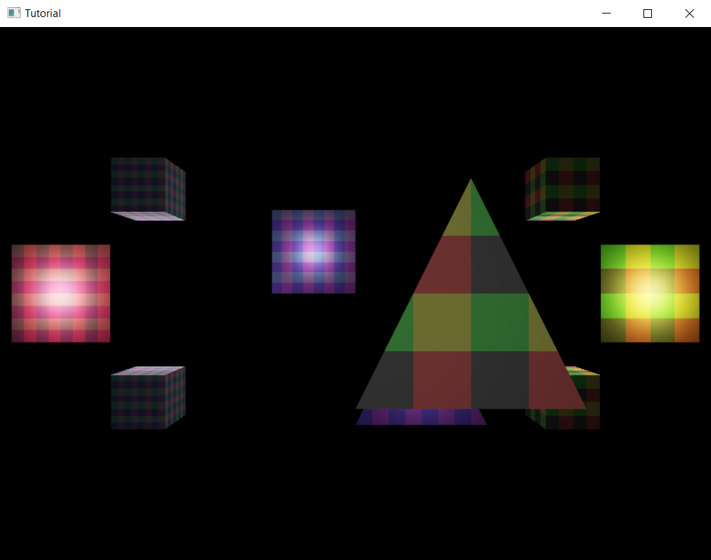
**Figure 11:** Screenshot of the application with diffuse lighting.

We have an application that can shade scene objects with diffuse lighting. We could end the tutorial here, but we should add a few extra pieces of functionality to our application.

Bonus: Draw a sphere

Let's add a new model, a sphere, to have another model to test our shaders. Then let's add a few scene objects that use this model. Spheres are useful because they will have a lot of surface elements with lots of normals pointing in a lot of directions, and you can observe how lighting affects them.

Sphere model

Let's write a few functions that will be the building blocks of generating a sphere model. The two functions will be linear interpolation and spherical linear interpolation. Both of them take two vectors and create a new vector "in-between", and they have a lot of applications in computer graphics, so it's a good idea to add them to your toolset.

Linear interpolation or LERP is a technique to create new point between two points by taking their weighted sum. Taking the weighted sum of two points results in a new point that is on the line that connects the two points.

When we generate our sphere we will use LERP to generate texture coordinates for our sphere points, so we implement it for 2D vectors. The implementation is below.


fn lerp(v1: [f32;2], v2: [f32;2], x:f32) -> [f32;2]
{
    [
        v1[0] * x + v2[0] * (1.0 - x),
        v1[1] * x + v2[1] * (1.0 - x)
    ]
}

We have a function that can create points in-between two points along a line. We could create points on a unit sphere's patch by linearly interpolating two points and normalizing the vectors, but those vectors would not be spaced evenly along the sphere surface, and this would look weird. This is where another interpolation technique comes in.

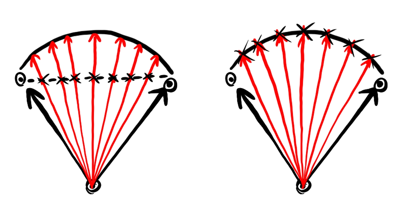
**Figure 12:** Illustration of the unevenness of circular arc samples. On the left you can see the vectors being linearly interpolated and then normalized. What was evenly spaced along a straight line will not be evenly spaced along a circular arc. The angles between them will be uneven, and as a result, the arclength between them will be uneven as well. On the right you can see vectors sampled along the circular arc with even arclength between them as comparison.

Spherical linear interpolation or SLERP is a method for creating a new point between two points along a circular arc. The parameter of the arc moves with constant angular velocity. The formula for SLERP is below.

slerp (p0, p1, t) = \frac{\sin ((1 - t) \cdot Ω)}{\sin (Ω)} \cdot p0 - \frac{\sin (t \cdot Ω)}{\sin (Ω)} \cdot p1

Where $p0$ and $p1$ are the interpolated points and $Ω$ is the angle between them.

SLERP has a page on wikipedia.

An implementation which assumes that the interpolated vectors are unit vectors is below.


fn slerp(v1: [f32;3], v2: [f32;3], x:f32) -> [f32;3]
{
    let dot = v1[0]*v2[0] + v1[1]*v2[1] + v1[2]*v2[2];
    let angle = dot.acos();

    let sin_angle = angle.sin();
    let weight1 = ((1.0 - x) * angle).sin() / sin_angle;
    let weight2 = (x * angle).sin() / sin_angle;
    [
        v1[0] * weight1 + v2[0] * weight2,
        v1[1] * weight1 + v2[1] * weight2,
        v1[2] * weight1 + v2[2] * weight2
    ]
}

Notice that without any normalization we dot the vectors together, and just take the result's acos. This only works for unit vectors!

Since the parameter moves with constant angular velocity, evenly spaced parameters will imply evenly spaced angles between the generated points, and it generates points along a circular arc, so this gets us closer to generating sphere patches.

Now we are going to generate sphere patches between four points. These points must be represented by a unit vector, so they must be points on the unit sphere. The idea is interpolating two edges facing each other with SLERP using one parameter, and interpolate these two points again with SLERP using another parameter. This results in a parametric equation of a sphere patch with two parameters.

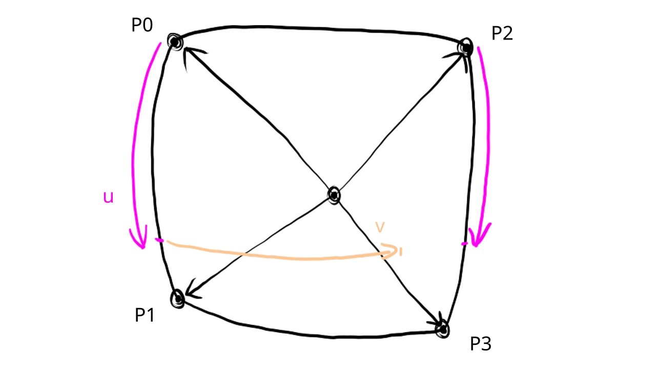
**Figure 13:** Illustration of a sphere patch. Two of the edges facing each other are constructed by SLERPing two vertices using the $u$ parameter, and the arc between every two point corresponding to the $u$ parameter is constructed by SLERPing them with the parameter $v$ . This creates a 2D parametric surface representing a sphere patch.

Texture coordinates are also supplied for every corner of the sphere patch, and they will be linearly interpolated.

Since the positions will be on the unit sphere, they can function as normal vectors, so we place them right after the position according to the memory layout of the vertex attributes defined during pipeline creation.

We determine the resolution using two integer parameters.

The implementation can be seen below.


fn create_sphere_patch_vertices_with_normals(
    positions: &[[f32;3];4],
    texcoords: &[[f32;2]; 4],
    resolution_x: usize,
    resolution_y: usize,
    vertices: &mut Vec<f32>
)
{
    let dx = (1.0)/(resolution_x - 1) as f32;
    let dy = (1.0)/(resolution_y - 1) as f32;
    for i in 0..resolution_x
    {
        let positions1 = slerp(positions[0], positions[1], i as f32 * dx);
        let positions2 = slerp(positions[2], positions[3], i as f32 * dx);
        let texcoord1  = lerp(texcoords[0], texcoords[1], i as f32 * dx);
        let texcoord2  = lerp(texcoords[2], texcoords[3], i as f32 * dx);

        for j in 0..resolution_y
        {
            let position = slerp(positions1, positions2, j as f32 * dy);
            let texcoord = lerp(texcoord1, texcoord2, j as f32 * dy);
            vertices.push(position[0]);
            vertices.push(position[1]);
            vertices.push(position[2]);
            vertices.push(position[0]);
            vertices.push(position[1]);
            vertices.push(position[2]);
            vertices.push(texcoord[0]);
            vertices.push(texcoord[1]);
        }
    }
}

We iterate over every sample point. In the outer loop we sample the two edges facing each other along the circular arc connecting them, then in the inner loop we sample the circular arc connecting these two points. We interpolate the texture coordinates following similar principles, but linearly. Then we push the position once into the output array to serve as position, then we push it again to serve as normal vector, and then we push the texture coordinates.

The vertices are laid out in memory row by row, one row after the other. With this layout the index buffer will be the following:


fn create_sphere_patch_indices(
    resolution_x: usize,
    resolution_y: usize,
    base_vertex: u32,
    indices: &mut Vec<u32>
)
{
    for i in 0..(resolution_x - 1)
    {
        for j in 0..(resolution_y - 1)
        {
            let next_i = i+1;
            let next_j = j+1;

            indices.push(base_vertex + (i*resolution_x + j) as u32);
            indices.push(base_vertex + (i*resolution_x + next_j) as u32);
            indices.push(base_vertex + (next_i*resolution_x + j) as u32);
            indices.push(base_vertex + (next_i*resolution_x + j) as u32);
            indices.push(base_vertex + (i*resolution_x + next_j) as u32);
            indices.push(base_vertex + (next_i*resolution_x + next_j) as u32);
        }
    }
}

We take the resolution along the two sides and a base vertex as parameters. The base vertex allows us to assemble a single model from multiple sphere patches laid out one after the other in memory, which we will take advantage of when generating a whole sphere.

Now that we can generate vertex and index data for a sphere patch, we can generate a sphere by generating multiple sphere patches.

**Figure 14:** Illustration of a sphere assembled from sphere patches.

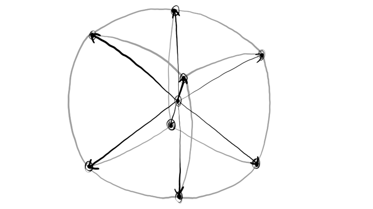
We define six sphere patches, one for the positive and negative X direction, one for the positive and negative Y direction, and one for the positive and negative Z direction. Neighboring patches will have the same corners. We generate a sphere patch with the given resolution for every one of them, we place them in the result array one after the other, and this will create a sphere.


fn create_sphere_vertices_with_normals(resolution_x: usize, resolution_y: usize) -> Vec<f32>
{
    let vec_len = 3.0_f32.sqrt();

    let pos_z = [
        [ 1.0 / vec_len, -1.0 / vec_len,  1.0 / vec_len],
        [-1.0 / vec_len, -1.0 / vec_len,  1.0 / vec_len],
        [ 1.0 / vec_len,  1.0 / vec_len,  1.0 / vec_len],
        [-1.0 / vec_len,  1.0 / vec_len,  1.0 / vec_len]
    ];

    let neg_z = [
        [-1.0 / vec_len, -1.0 / vec_len, -1.0 / vec_len],
        [ 1.0 / vec_len, -1.0 / vec_len, -1.0 / vec_len],
        [-1.0 / vec_len,  1.0 / vec_len, -1.0 / vec_len],
        [ 1.0 / vec_len,  1.0 / vec_len, -1.0 / vec_len]
    ];

    let pos_x = [
        [ 1.0 / vec_len, -1.0 / vec_len, -1.0 / vec_len],
        [ 1.0 / vec_len, -1.0 / vec_len,  1.0 / vec_len],
        [ 1.0 / vec_len,  1.0 / vec_len, -1.0 / vec_len],
        [ 1.0 / vec_len,  1.0 / vec_len,  1.0 / vec_len]
    ];

    let neg_x = [
        [-1.0 / vec_len, -1.0 / vec_len,  1.0 / vec_len],
        [-1.0 / vec_len, -1.0 / vec_len, -1.0 / vec_len],
        [-1.0 / vec_len,  1.0 / vec_len,  1.0 / vec_len],
        [-1.0 / vec_len,  1.0 / vec_len, -1.0 / vec_len]
    ];

    let pos_y = [
        [ 1.0 / vec_len,  1.0 / vec_len,  1.0 / vec_len],
        [-1.0 / vec_len,  1.0 / vec_len,  1.0 / vec_len],
        [ 1.0 / vec_len,  1.0 / vec_len, -1.0 / vec_len],
        [-1.0 / vec_len,  1.0 / vec_len, -1.0 / vec_len]
    ];

    let neg_y = [
        [-1.0 / vec_len, -1.0 / vec_len,  1.0 / vec_len],
        [ 1.0 / vec_len, -1.0 / vec_len,  1.0 / vec_len],
        [-1.0 / vec_len, -1.0 / vec_len, -1.0 / vec_len],
        [ 1.0 / vec_len, -1.0 / vec_len, -1.0 / vec_len]
    ];

    let texcoords = [
        [0.0, 0.0],
        [1.0, 0.0],
        [0.0, 1.0],
        [1.0, 1.0]
    ];

    let mut vertices = Vec::with_capacity(resolution_x * resolution_y);

    create_sphere_patch_vertices_with_normals(&pos_z, &texcoords, resolution_x, resolution_y, &mut vertices);
    create_sphere_patch_vertices_with_normals(&neg_z, &texcoords, resolution_x, resolution_y, &mut vertices);
    create_sphere_patch_vertices_with_normals(&pos_x, &texcoords, resolution_x, resolution_y, &mut vertices);
    create_sphere_patch_vertices_with_normals(&neg_x, &texcoords, resolution_x, resolution_y, &mut vertices);
    create_sphere_patch_vertices_with_normals(&pos_y, &texcoords, resolution_x, resolution_y, &mut vertices);
    create_sphere_patch_vertices_with_normals(&neg_y, &texcoords, resolution_x, resolution_y, &mut vertices);

    vertices
}

Then we calculate the indices of the sphere patches using the previous index generation function. We take advantage of the way the patches are laid out in memory, and bumping the base vertex will shift the index buffer of the sphere patches the right way.


fn create_sphere_indices(resolution_x: usize, resolution_y: usize) -> Vec<u32>
{
    let mut indices = Vec::with_capacity((resolution_x-1)*(resolution_y-1)*2*3);

    let mut base_vertex = 0;

    create_sphere_patch_indices(resolution_x, resolution_y, base_vertex as u32, &mut indices);
    base_vertex += resolution_x*resolution_y;

    create_sphere_patch_indices(resolution_x, resolution_y, base_vertex as u32, &mut indices);
    base_vertex += resolution_x*resolution_y;

    create_sphere_patch_indices(resolution_x, resolution_y, base_vertex as u32, &mut indices);
    base_vertex += resolution_x*resolution_y;

    create_sphere_patch_indices(resolution_x, resolution_y, base_vertex as u32, &mut indices);
    base_vertex += resolution_x*resolution_y;

    create_sphere_patch_indices(resolution_x, resolution_y, base_vertex as u32, &mut indices);
    base_vertex += resolution_x*resolution_y;

    create_sphere_patch_indices(resolution_x, resolution_y, base_vertex as u32, &mut indices);

    indices
}

Adding them to the scene

Now let's upload the model and add a few scene objects using it!

First we create the vertex and index data.


    //
    // Vertex and Index data
    //

    // ...

    let sphere_vertices = create_sphere_vertices_with_normals(16, 16);
    let sphere_indices = create_sphere_indices(16, 16);

    // Vertex and Index buffer size

    // ...

    let sphere_vertex_data_size = sphere_vertices.len() * core::mem::size_of::<f32>();
    let sphere_index_data_size = sphere_indices.len() * core::mem::size_of::<u32>();

    let vertex_data_size = tri_and_quad_vertex_data_size + cube_vertex_data_size + sphere_vertex_data_size;
    let index_data_size = tri_and_quad_index_data_size + cube_index_data_size + sphere_index_data_size;

We must also adjust the vertex and index buffer size as well.

Then we upload.



    //
    // Uploading to Staging buffer
    //

    // ...

    unsafe
    {
        // ...

        //
        // Copy vertex and index data to staging buffer
        //

        // ...

        // Cube vertex data

        // ...

        // Sphere vertex data

        let vertex_data_offset = vertex_data_offset + cube_vertex_data_size as isize;
        let vertex_data_void = data.offset(vertex_data_offset);
        let vertex_data_typed: *mut f32 = core::mem::transmute(vertex_data_void);
        core::ptr::copy_nonoverlapping::<f32>(
            sphere_vertices.as_ptr(),
            vertex_data_typed,
            sphere_vertices.len()
        );

        // ...

        // Cube index data

        // ...

        // Sphere index data

        let index_data_offset = index_data_offset + cube_index_data_size as isize;
        let index_data_void = data.offset(index_data_offset);
        let index_data_typed: *mut u32 = core::mem::transmute(index_data_void);
        core::ptr::copy_nonoverlapping::<u32>(
            sphere_indices.as_ptr(),
            index_data_typed,
            sphere_indices.len()
        );

        // ...
    }

Then we add it to the list of models.



    //
    // Model and Texture ID-s
    //

    // Models

    // ...
    let sphere_index = 3;

    let models = [
        // ...

        // Sphere
        Model {
            index_count: sphere_indices.len() as u32,
            first_index: (tri_and_quad_indices.len() + cube_indices.len()) as u32,
            vertex_offset: ((tri_and_quad_vertices.len() + cube_vertices.len()) / PER_VERTEX_DATA_SIZE) as i32
        }
    ];

Then we add a few scene elements.


    //
    // Game state
    //

    // ...

    // Game logic state

    // ...

    // Spheres added later

    static_meshes.push(
        StaticMesh {
            x: 2.0,
            y: 0.5,
            z: -2.5,
            scale: 0.25,
            rot_x: 0.0,
            rot_y: 0.0,
            albedo_r: 1.0,
            albedo_g: 1.0,
            albedo_b: 1.0,
            emissive_r: 0.0,
            emissive_g: 0.0,
            emissive_b: 0.0,
            texture_index: red_yellow_green_black_tex_index,
            model_index: sphere_index
        }
    );
    static_meshes.push(
        StaticMesh {
            x: 2.0,
            y: -0.5,
            z: -2.5,
            scale: 0.25,
            rot_x: 0.0,
            rot_y: 0.0,
            albedo_r: 1.0,
            albedo_g: 1.0,
            albedo_b: 1.0,
            emissive_r: 0.0,
            emissive_g: 0.0,
            emissive_b: 0.0,
            texture_index: red_yellow_green_black_tex_index,
            model_index: sphere_index
        }
    );
    static_meshes.push(
        StaticMesh {
            x: -2.0,
            y: 0.5,
            z: -2.5,
            scale: 0.25,
            rot_x: 0.0,
            rot_y: 0.0,
            albedo_r: 1.0,
            albedo_g: 1.0,
            albedo_b: 1.0,
            emissive_r: 0.0,
            emissive_g: 0.0,
            emissive_b: 0.0,
            texture_index: blue_cyan_magenta_white_tex_index,
            model_index: sphere_index
        }
    );
    static_meshes.push(
        StaticMesh {
            x: -2.0,
            y: -0.5,
            z: -2.5,
            scale: 0.25,
            rot_x: 0.0,
            rot_y: 0.0,
            albedo_r: 1.0,
            albedo_g: 1.0,
            albedo_b: 1.0,
            emissive_r: 0.0,
            emissive_g: 0.0,
            emissive_b: 0.0,
            texture_index: blue_cyan_magenta_white_tex_index,
            model_index: sphere_index
        }
    );

If we run the application now, a few spheres will be added and we can observe how diffuse lighting works on them. They are excellent testing data and I highly recommend them.

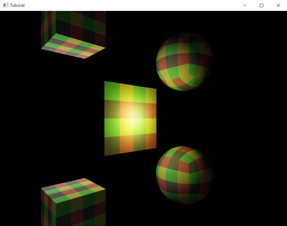
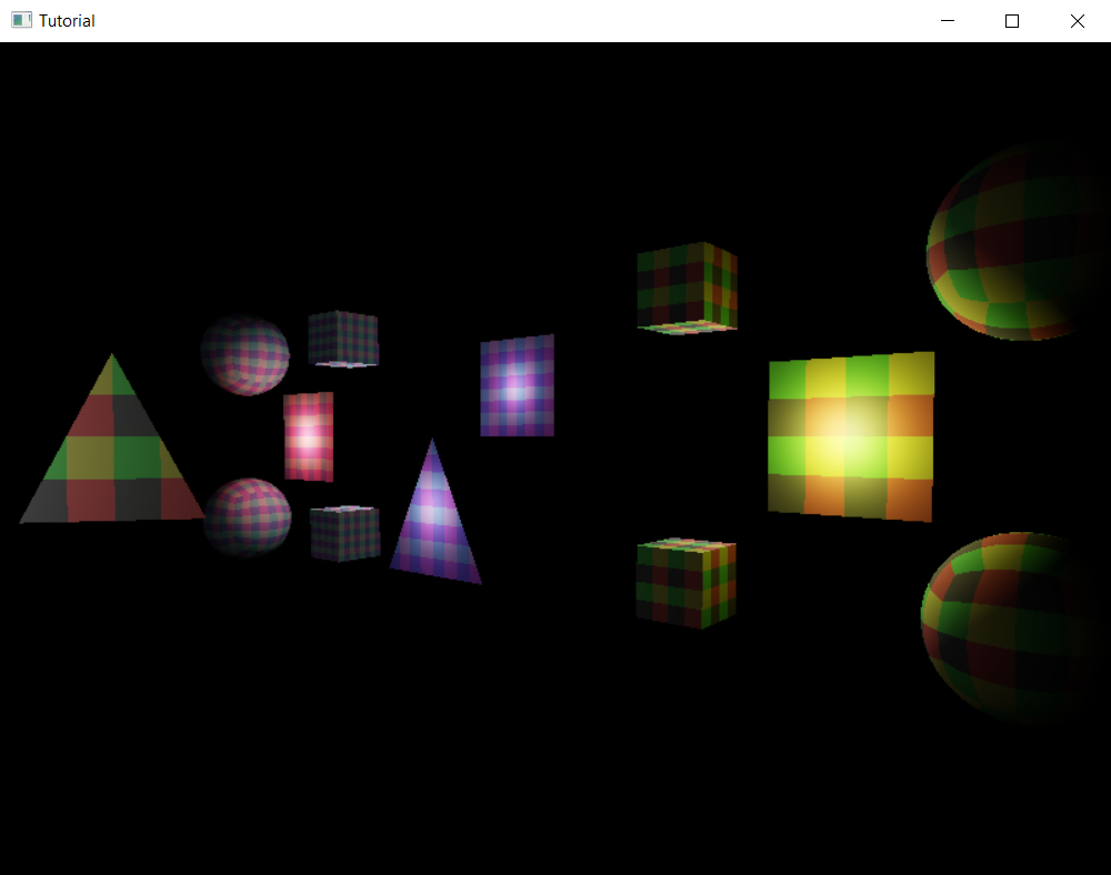
**Figure 15:** Screenshot of the application with sphere models. The result of interpolating normals for lighting calculations is clearly visible, as it does not look like it's assembled from flat triangles like the cube model.

I could conclude the tutorial, but no. I want you to use this sphere model to implement a useful debug feature to visualize light sources. :) It's going to give you some fun ideas, so let's get started!

Representing lights with spheres

Let's draw a small emissive sphere everywhere where we have a point light!

I want to put some ideas into your head. For static meshes we basically had a straightforward mapping between the scene element's data and the uniform buffer regions. For point lights the mapping will be less straightforward. We will have some artistic freedom. Maybe in your own game you will have interesting scene elements where the source data is also not a 1:1 mapping with the uniform buffer regions, and understanding that scene data can be derived from game state in creative ways will give you some interesting ideas.

Let's add point_light_radius somewhere where it makes sense!


    //
    // Game state
    //

    // ...

    // Game logic state

    // ...

    let point_light_radius = 0.0125;

    // ...

Now let's upload transforms and material data that makes sense for every point light!


        //
        // Uniform upload
        //

        {
            // Getting references

            // ...

            // Filling them with data

            // ...

            let light_transform_data_array = &mut transform_data_array[static_meshes.len()..static_meshes.len() + lights.len()];
            for (i, light) in lights.iter().enumerate()
            {
                light_transform_data_array[i] = core::mem::MaybeUninit::new(
                    TransformData {
                        model_matrix: mat_mlt(
                            &translate(
                                light.x,
                                light.y,
                                light.z
                            ),
                            &scale(
                                point_light_radius,
                                point_light_radius,
                                point_light_radius
                            )
                        )
                    }
                );
            }

            let light_material_data_array = &mut material_data_array[static_meshes.len()..static_meshes.len() + lights.len()];
            for (i, light) in lights.iter().enumerate()
            {
                let mlt = 1.0 / (point_light_radius * point_light_radius);
                light_material_data_array[i] = core::mem::MaybeUninit::new(
                    MaterialData {
                        albedo: [
                            0.0,
                            0.0,
                            0.0,
                            0.0
                        ],
                        emissive: [
                            light.intensity_r * mlt,
                            light.intensity_g * mlt,
                            light.intensity_b * mlt,
                            0.0
                        ]
                    }
                );
            }
        }

A transform that translates the sphere model to the position of the point light and scales it to the radius we chose makes sense. Also a material data that emits the radiant intensity with an inverse square falloff makes sense, after all one of our assumptions at the beginning of the chapters was that the radiant intensity gets evenly distributed in every direction.

Then let's encode rendering commands! We want to draw a sphere with our newly uploaded transform and material data for every point light.


        //
        // Rendering commands
        //

        // ...

        unsafe
        {
            vkCmdBeginRenderPass(
                cmd_buffers[current_frame_index],
                &render_pass_begin_info,
                VK_SUBPASS_CONTENTS_INLINE
            );

            // ...

            // Setting texture descriptor array index For lights it is irrelevant.
            let texture_index: u32 = 0;
            vkCmdPushConstants(
                cmd_buffers[current_frame_index],
                pipeline_layout,
                VK_SHADER_STAGE_FRAGMENT_BIT as VkShaderStageFlags,
                2 * core::mem::size_of::<u32>() as u32,
                core::mem::size_of::<u32>() as u32,
                &texture_index as *const u32 as *const core::ffi::c_void
            );

            for light_obj_index in static_meshes.len()..(static_meshes.len() + lights.len())
            {
                // Per obj array index
                let object_index = light_obj_index as u32;

                vkCmdPushConstants(
                    cmd_buffers[current_frame_index],
                    pipeline_layout,
                    (VK_SHADER_STAGE_VERTEX_BIT | VK_SHADER_STAGE_FRAGMENT_BIT) as VkShaderStageFlags,
                    0,
                    core::mem::size_of::<u32>() as u32,
                    &object_index as *const u32 as *const core::ffi::c_void
                );

                vkCmdDrawIndexed(
                    cmd_buffers[current_frame_index],
                    models[sphere_index].index_count,
                    1,
                    models[sphere_index].first_index,
                    models[sphere_index].vertex_offset,
                    0
                );
            }

            vkCmdEndRenderPass(
                cmd_buffers[current_frame_index]
            );
        }

...and now really that's it! Now the application looks a bit cuter, and more of the scene's structure is communicated to you visually.

**Figure 17:** Screenshot of the application with emissive spheres indicating point lights.

Related: Postprocessing

In this tutorial we performed exposure correction, tone mapping and sRGB conversion at the end of the fragment shader for the sake of simplicity and because this tutorial was already massive, however it's conventional to first render the scene into an image, and apply exposure correction, tone mapping, sRGB conversion and many other things like bloom in a series of comupte shaders, and write the results to the swapchain image from there. This is called postprocessing.

We could get away without it, because we use a manually set exposure value, and because of this post processing could be done locally for every pixel, however, more advanced postprocessing techniques such as eye adaptation and bloom require the whole image to be rendered, because their operations require aggregate data of the whole image or access to neighboring pixels. In those cases you have no choice but to add a postprocessing step.

The first chapter in this tutorial where we will need to separate the postprocessing step will be the eye adaptation chapter.

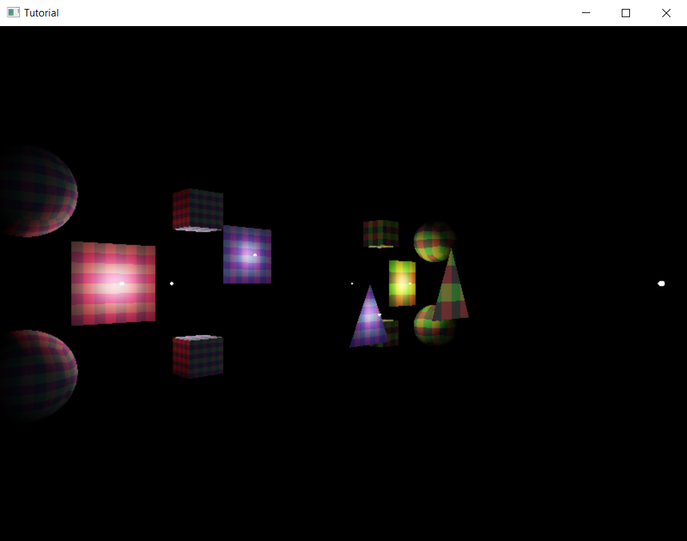
Wrapping up

In this chapter we laid down the foundations for physically based rendering. We learned about the rendering equation, simplified it until it became suitable for execution on the GPU, and learned the postprocessing steps (exposure correction, tone mapping and sRGB conversion) required to output the results of our simulation to the swapchain image.

We have extended our scene representation to include all the information necessary, such as surface normals, material data and point lights, and implemented a simulation based on the theory we learned at the beginning.

In the rest of the chapters in the PBR tutorial we will extend this foundation with specular lighting, environment mapping and many other useful features.

The sample code for this tutorial can be found here.

The tutorial continues here.